
Week 5CHAPTER 05
Valuation Methods for Startups
The capstone of the valuation sequence, turning the Week 4 forecast into a defensible number across every professional method. Why every valuation answers one question and how the income, market, and cost approaches triangulate; the DCF engine from FCFF and FCFE to enterprise and equity value; building the discount rate with CAPM and WACC (and the circularity problem); terminal value via the Gordon Growth Model and exit multiples; IRR, its hidden reinvestment flaw, and MIRR; stage-adjusted year-by-year discount rates; the market lens of trading comparables and precedent transactions; the VC method and future-dilution math; the cost approach as a floor; how deal terms diverge from headline valuation; probability-weighted scenario value; and triangulating every method into a football-field range, with seven interactive calculators.
~140 min8 sections52 questions8 tools
Learning objectives (9)
Learning Objectives
By the end of this chapter you should be able to:
- 1Explain why valuation ultimately answers one question (what a specific buyer will pay a specific seller at a specific time) and how the income, market, and cost approaches triangulate.
- 2Build a discounted cash flow valuation from free cash flow, distinguishing FCFF (discounted at WACC to enterprise value) from FCFE (discounted at the cost of equity to equity value).
- 3Construct a discount rate using the CAPM cost of equity and WACC, add a size premium for small firms, and recognize the circularity problem in WACC.
- 4Estimate terminal value with the Gordon Growth Model and the exit multiple method, and interpret why terminal value is typically 60 to 80% of enterprise value.
- 5Compute and compare IRR and MIRR, and explain the reinvestment-rate assumption and the multiple-IRR problem that MIRR resolves.
- 6Apply stage-adjusted, year-by-year discount rates that decline as venture risk resolves, rather than a single flat rate.
- 7Value a company with the market approach using trading comparables and precedent transactions, and avoid the common selection pitfalls.
- 8Apply the VC method to work backward from a projected exit at a target return, and adjust the required ownership for future dilution.
- 9Use the cost approach as a floor, distinguish valuation from deal economics, and combine probability-weighted scenarios and triangulation into a defensible value range.
Part One: Every Valuation Answers One Question. Section 1 of 8.
Part One · Every Valuation Answers One Question
Every Valuation Answers One Question
Converting an uncertain future into a present-day price
Valuation is the act of converting an uncertain future into a present-day price. Every method, model, and back-of-napkin estimate is a version of the same exercise: project what an asset will produce, adjust for risk, and express the result in today's dollars. The differences between methods are differences of inputs, assumptions, and which risks receive explicit treatment versus which get buried in a single number.
The three master approaches
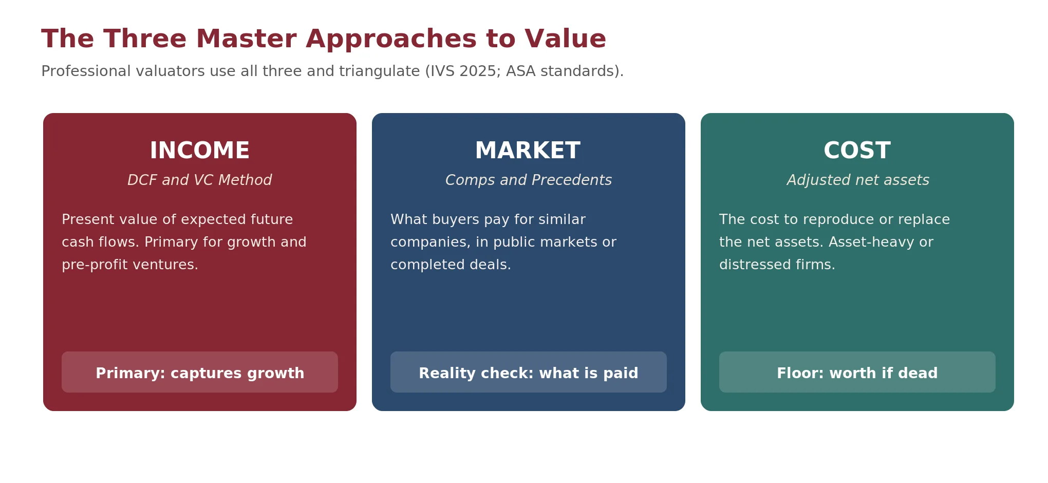
Professional valuators organize their work into three master approaches, codified in the International Valuation Standards (IVS, effective 31 January 2025) and the American Society of Appraisers Business Valuation Standards. The income approach values the business as the present value of expected future cash flows, with DCF as the primary tool. It is central to venture analysis because a venture's value lies almost entirely in future cash flows that do not yet exist. The market approach values the business by reference to what similar businesses have sold for, in public trading markets or completed transactions. It is observational: it tells you what buyers have paid, not what the asset is intrinsically worth. The cost approach values the business at the cost to reproduce or replace its underlying assets, relevant for asset-heavy or distressed businesses and rarely primary for operating companies with intangible value.
| Approach | Best when |
|---|---|
| Income (DCF, VC method) | Future cash flows are the primary source of value; the company is growing or pre-profit |
| Market (comps, precedents) | Sufficient comparable companies exist and you need a market-grounded sanity check |
| Cost (adjusted net assets) | Asset-heavy business, a liquidation scenario, an IP portfolio, or a holding company |
For entrepreneurial ventures, the income approach is primary because it captures future growth. The market approach provides a reality check on what investors are actually paying. The cost approach sets a floor, what the business is worth if broken up. Professionals use all three and triangulate.
Check Your Understanding
Knowledge Check 1
Valuation & DCF
In valuing an early-stage venture, how do the three master valuation approaches (income, market, and cost) generally fit together?
The Discounted Cash Flow Model
The Discounted Cash Flow model is the analytical core of income-based valuation. It has two variants, distinguished by which cash flow they measure and which discount rate they apply. Knowing when to use each is a core skill for those building or evaluating a model.
Free Cash Flow to the Firm (FCFF)
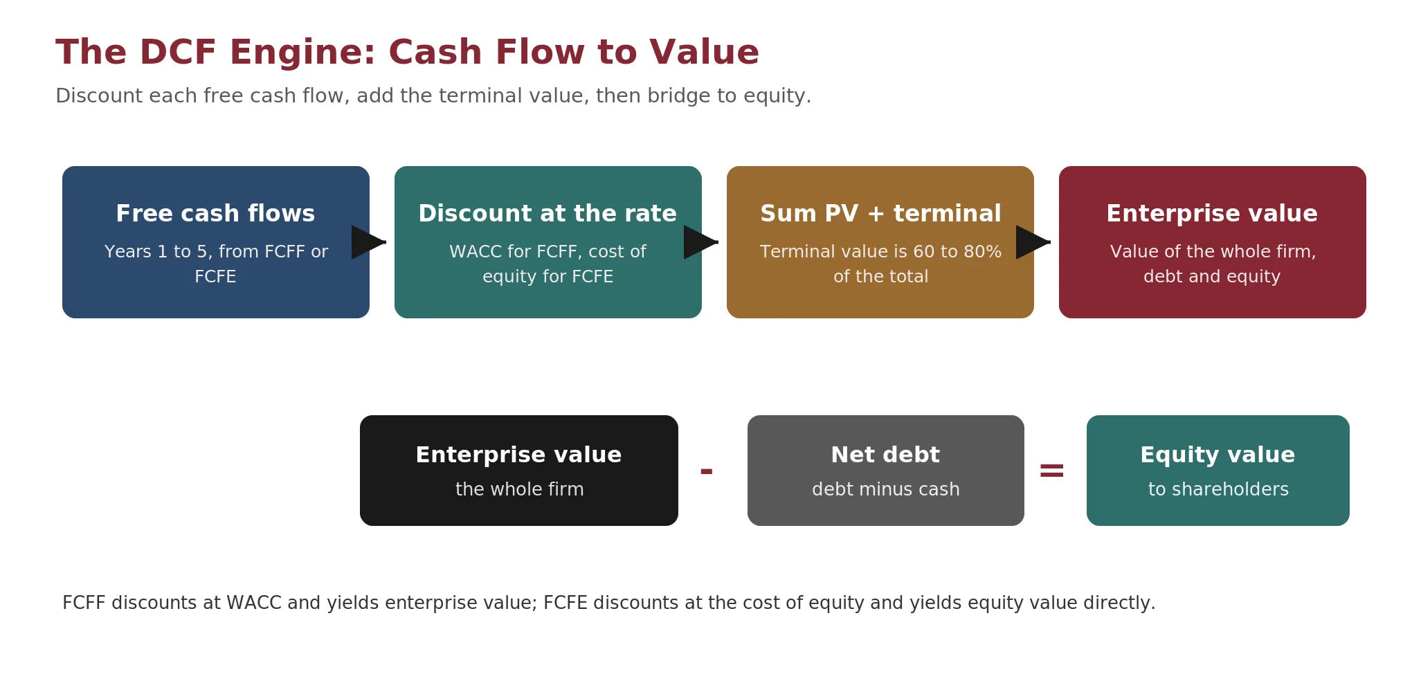
FCFF measures the cash available to all capital providers, debt and equity, after the business funds operations and reinvestment. It is the cash the entire enterprise generates before any financing decisions.
Formula. FCFF = NOPAT + Depreciation & Amortization - Capital Expenditures - Increase in Net Working Capital, where NOPAT = EBIT x (1 - Tax Rate)
NOPAT strips out interest expense because FCFF is pre-financing; the cost of debt is captured in the discount rate, WACC, not in the cash flow. Discounting FCFF at WACC produces enterprise value, the value of the whole firm. To reach equity value, subtract net debt (total debt minus cash).
Free Cash Flow to Equity (FCFE)
FCFE measures the cash available to equity holders specifically, after the business pays its debt obligations. It accounts for actual interest payments and net borrowing.
Formula. FCFE = Net Income + D&A - CapEx - Increase in NWC + Net Borrowing
Discount FCFE at the cost of equity, not WACC, and it yields equity value directly, with no need to subtract debt. Use FCFF when the capital structure will change significantly, when comparing companies with different leverage, or in standard investment-banking and M&A work. Use FCFE when the capital structure is stable, when valuing a single company with predictable debt service, or for banks and financial institutions.
Worked Example: An FCFF Calculation
A SaaS company reports EBIT of $5M, a 25% tax rate, D&A of $0.8M, CapEx of $1.2M, and a $0.3M year-over-year increase in net working capital. NOPAT is $5M x (1 - 0.25) = $3.75M. FCFF is $3.75M + $0.8M - $1.2M - $0.3M = $3.05M. If WACC is 10%, this single year's FCFF contributes $3.05M / 1.10 = $2.77M of present value to enterprise value.
Set EBIT to $5M at a 25% tax rate, with D&A of $0.8M, CapEx of $1.2M, and a $0.3M working-capital increase, to reproduce a benchmark FCFF of $3.05M, then move each lever to see how FCFF and FCFE respond.
Check Your Understanding
Knowledge Check 2
Valuation & DCF
You discount FCFF in a DCF. Which rate applies, and what result do you get?
Knowledge Check 3
Valuation & DCF
EBIT is $5M, tax rate 25%, D&A $0.8M, CapEx $1.2M, and net working capital rose $0.3M. What is FCFF?
Part Three
Building the Discount Rate: CAPM, WACC, and What They Miss
The discount rate is typically the single most consequential input in a DCF. A 2% change in the rate can shift a valuation by 30 to 50% or more. Understanding how it is built, and where it breaks down, is essential.
The Capital Asset Pricing Model
Sharpe (1964) and Lintner (1965) developed CAPM as the foundational model for the cost of equity. Investors demand compensation for the risk-free time value of money plus a premium proportional to the systematic, non-diversifiable risk the investment carries.
Formula. Cost of Equity = Risk-Free Rate + Beta x (Market Return - Risk-Free Rate)
The risk-free rate is a government bond yield matching the cash-flow horizon, typically the 10-year US Treasury (near 4.3% as of early 2026). Beta measures sensitivity to the market: 1.0 moves with the market, 1.5 is 50% more volatile. For private companies, use unlevered betas of comparable public firms, then re-lever for the target's capital structure. The equity risk premium is the excess return investors demand for equities over risk-free bonds; Damodaran's implied ERP for the US market was 4.23% as of January 2026, derived from current S&P 500 prices and forward cash-flow expectations. Treat both the risk-free rate and the ERP as as-of-date figures that will change.
Check Your Understanding
Knowledge Check 4
Cost of Capital (WACC) & VC Method
The risk-free rate is 4%, beta is 1.2, and the equity risk premium is 5%. What is the CAPM cost of equity?
The Fama-French Three-Factor Model
Fama and French (1993) showed that CAPM's single market factor leaves substantial return variation unexplained. Adding a size premium (SMB, Small Minus Big) and a value premium (HML, High Minus Low) materially improves explanatory power across most equity samples tested. The magnitude varies by geography and period, but the three-factor model is the standard academic benchmark for expected returns.
Formula. E(R) = Risk-Free Rate + b1 x Market Premium + b2 x SMB + b3 x HML
For entrepreneurial finance, the size premium matters most. Small-capitalization firms have historically earned higher returns, compensating for higher risk, lower liquidity, and greater information asymmetry. When valuing a startup or small private company, adding a size premium of roughly 2 to 6% on top of CAPM produces a more realistic cost of equity. Treat that band as a practitioner range, not a precise constant.
Assembling WACC
Formula. WACC = (E/V) x Cost of Equity + (D/V) x Cost of Debt x (1 - Tax Rate), where V = E + D
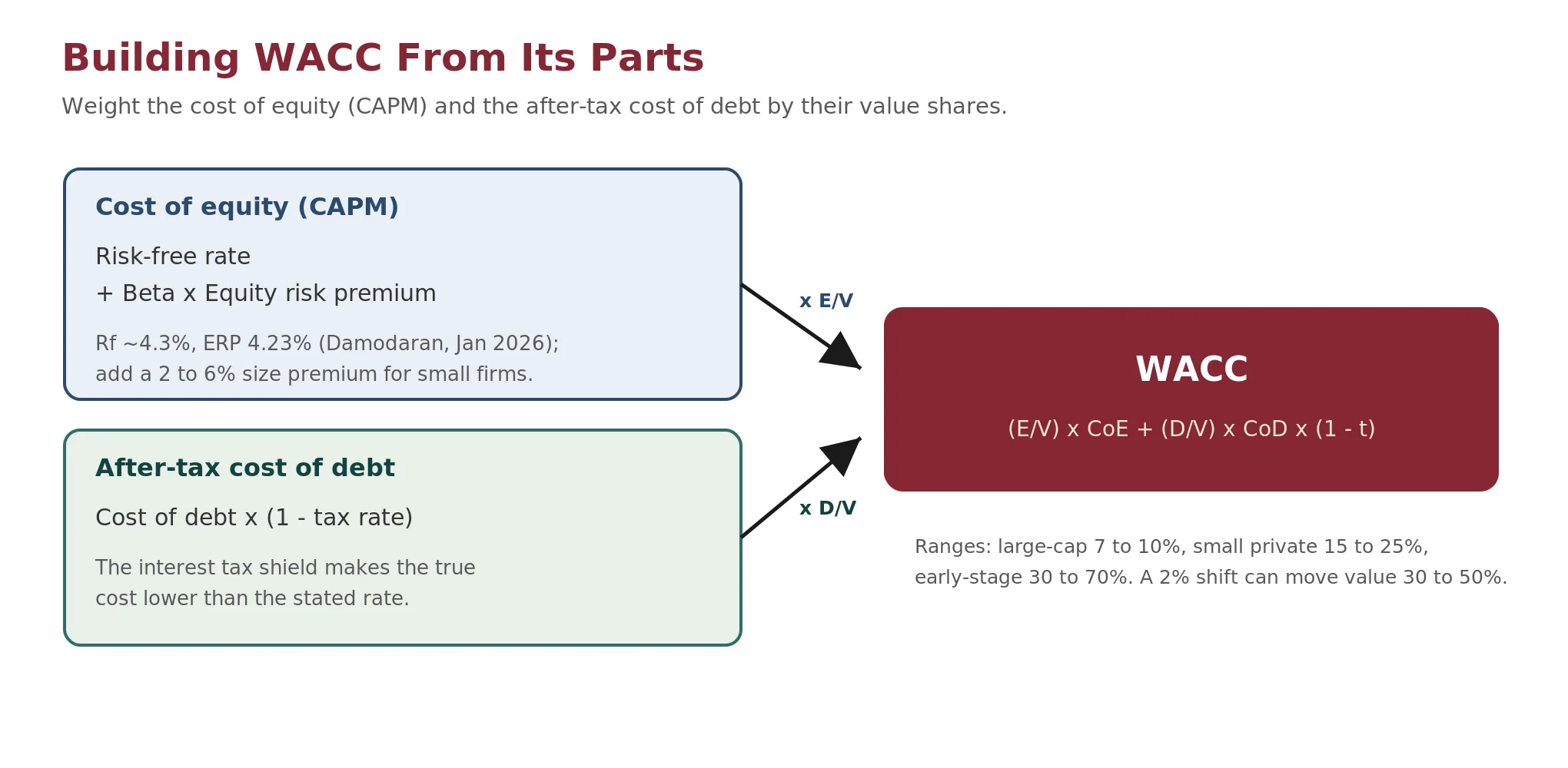
The after-tax cost of debt reflects the interest tax shield: because interest is tax-deductible, the true cost of debt is lower than the stated rate. Typical WACC ranges, as practitioner rules of thumb, run 7 to 10% for large-cap stable companies, 10 to 14% for mid-cap growth, 15 to 25% for small private companies, and 30 to 70% for early-stage ventures, if DCF is used at all.
Worked example
Take the CAPM cost of equity from above, 10%, for a company financed 70% equity and 30% debt, with a pre-tax cost of debt of 8% and a 21% tax rate. The after-tax cost of debt is 8% × (1 − 0.21) = 6.3%. WACC is then 0.70 × 10% + 0.30 × 6.3% = 7.0% + 1.9% = 8.9%. Notice the debt contributes only 1.9 points, both because it is the smaller weight and because the tax shield lowers its effective cost from 8% to 6.3%.
Adjust the CAPM inputs and capital-structure weights to see the cost of equity and WACC. The defaults reproduce the worked example above (Rf 4%, β 1.2, ERP 5% → cost of equity 10%; 70/30 weights, 8% debt, 21% tax → WACC 8.9%).
The Circularity Problem
WACC requires the market value of equity to compute E/V, but the market value of equity is exactly what the DCF is trying to solve for. This is a circular reference. Three solutions exist.
- First, iterative calculation: assume an initial capital structure, run the DCF, check whether the resulting equity value reproduces the same weights, and iterate to convergence, which modern spreadsheets automate.
- Second, a target capital structure: use management's target or the industry average, treating capital structure as a policy choice rather than a market observation.
- Third, Adjusted Present Value: Myers (1974) proposed valuing the firm as if all-equity financed, discounting FCFF at the unlevered cost of equity, then separately adding the present value of the interest tax shield. APV eliminates the circularity entirely because it does not use WACC.
Check Your Understanding
Knowledge Check 5
Cost of Capital (WACC) & VC Method
WACC needs the market value of equity, but that is what the DCF solves for. Which method avoids the circularity entirely?
Terminal Value: The Tail That Wags the Dog
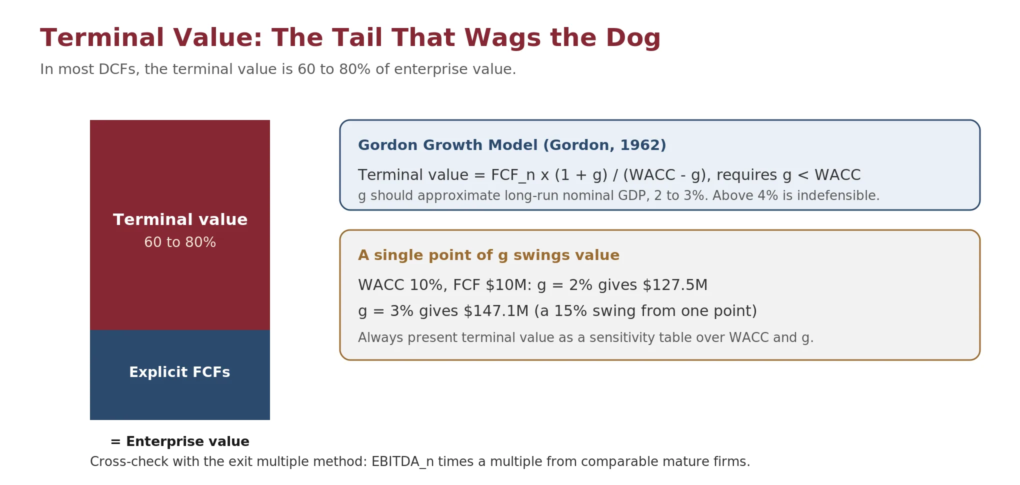
A DCF typically forecasts explicit cash flows for 5 to 10 years, then estimates the value of everything beyond that horizon as a single lump sum, the terminal value. In most valuations, terminal value is 60 to 80% of total enterprise value. The majority of the valuation therefore depends on assumptions about what happens after the detailed forecast ends. Handle this with extreme care.
Method 1: The Gordon Growth Model
Gordon (1962) treats post-forecast cash flows as a perpetuity growing at a constant rate forever.
Formula. Terminal Value = FCF_n x (1 + g) / (WACC - g), which requires g < WACC
FCF_n is the final year's free cash flow, g is the perpetuity growth rate, and WACC is the discount rate. The formula requires g below WACC; otherwise it produces a negative or infinite value, signaling internally inconsistent assumptions. This produces the terminal value as of Year n, so to incorporate it you discount it back to the present.
Formula. PV of Terminal Value = Terminal Value / (1 + WACC)^n, and Enterprise Value = Sum of PV(explicit FCFs) + PV of Terminal Value
Keep the two components visible; the split reveals how much of the valuation rests on near-term projections versus the perpetuity assumption. The perpetuity growth rate should approximate long-run nominal GDP growth, typically 2 to 3% for developed economies. A company rarely outgrows the broader economy for long, so using g above 4% is generally indefensible. Sensitivity matters enormously: with WACC of 10% and FCF of $10M, changing g from 2% to 3% raises terminal value from $127.5M to $147.1M, a 15% swing from one percentage point. As a rule, present terminal value in a sensitivity table across WACC and g.
Adjust the final-year free cash flow, WACC, and perpetuity growth rate to see the Gordon Growth terminal value. The defaults reproduce a standard worked example (FCF $10M, WACC 10%, g 2% → $127.5M).
Check Your Understanding
Knowledge Check 6
Valuation & DCF
Final-year FCF is $10M, WACC is 10%, and perpetuity growth is 3%. What is the terminal value at Year n?
Method 2: The Exit Multiple Method
Instead of assuming perpetual growth, apply a valuation multiple to the final year's metric, typically EBITDA or revenue.
Formula. Terminal Value = EBITDA_n x Exit Multiple
The exit multiple is usually derived from current trading multiples of comparable mature companies, on the logic that the firm will have matured by the end of the forecast. The advantage is that it is intuitive and anchored to observable data. The disadvantage is that it embeds current market conditions into a future exit: if today's multiples are inflated by a bubble, the terminal value inflates too. Best practice is to compute terminal value both ways and compare. If the Gordon result exceeds the exit-multiple result, the perpetuity growth may be too aggressive. If the exit multiple exceeds Gordon, the market may be pricing in optionality that a steady-state model misses, or WACC is too high.
Check Your Understanding
Knowledge Check 7
Valuation & DCF
In a typical DCF, roughly what share of enterprise value comes from the terminal value?
The Reinvestment Rate Assumption
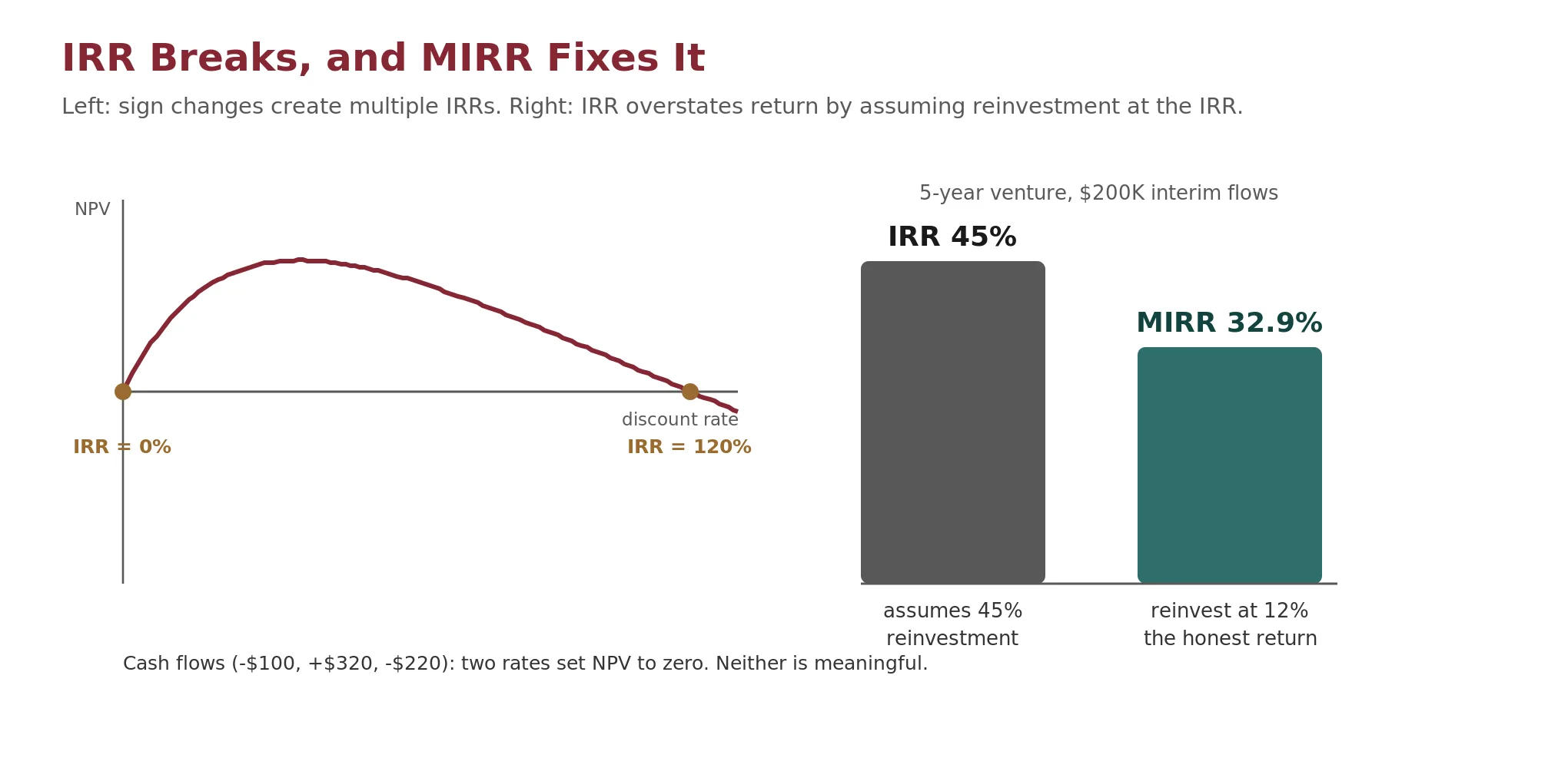
Using IRR to rank compound returns implicitly assumes that all interim cash flows can be reinvested at the IRR itself. If a project's IRR is 35%, comparing on that basis assumes every dollar of interim cash earns 35% from receipt to the end of the horizon. The formula does not literally reinvest anything, but the moment you use IRR to rank projects or to equate an IRR with a realized compound return, you have made this assumption. It is rarely realistic. A distribution from an early exit does not automatically earn 35%; it sits in a money market at 4 to 5% or gets recycled into a new deal with its own risk. The higher the IRR, the more the assumption inflates the reported return relative to actual wealth accumulation.
Check Your Understanding
Knowledge Check 8
Fund Returns (IRR, MOIC, J-Curve, Power Law)
Why can IRR overstate an investment's realized return when the IRR is very high?
The Multiple-IRR Problem
When cash flows switch signs more than once, the IRR equation can produce several valid solutions. Consider an investment with cash flows of minus $100, plus $320, and minus $220. Solving the NPV equation yields two valid IRRs, 0% and 120%. Neither is wrong mathematically, but neither is economically meaningful. The project changes direction twice, which is the situation where a single IRR breaks down.
Modified IRR: The Fix
MIRR addresses both problems by requiring two explicit rates: a finance rate for funding negative cash flows (typically the cost of capital) and a reinvestment rate for positive interim cash flows (typically WACC or a conservative market return). MIRR compounds all inflows forward to the terminal date at the reinvestment rate, discounts all outflows back to time zero at the finance rate, then solves for the single rate connecting them. This yields a unique solution and reflects realistic reinvestment.
Formula. MIRR = (Terminal Value of Inflows / PV of Outflows)^(1/n) - 1
Worked Example: IRR Versus MIRR
A venture has cash flows over five years of minus $500K, then plus $200K, plus $200K, plus $200K, plus $200K, and plus $1,000K. Traditional IRR is 45.0%. Now assume interim distributions reinvest at 12%, not 45%. The terminal value of inflows at 12% is $200K x 1.574 + $200K x 1.405 + $200K x 1.254 + $200K x 1.120 + $1,000K = $2,070.6K. The present value of outflows is $500K at time zero. MIRR is ($2,070.6K / $500K) to the 1/5 power, minus 1, which is (4.141) to the 0.2 power, minus 1, or 32.9%. The MIRR is 12 points below the IRR because interim cash does not earn 45% after distribution. MIRR gives a truer picture of actual wealth accumulation.
| Use IRR when | Use MIRR when |
|---|---|
| One outflow and one terminal inflow | There are multiple interim distributions before exit |
| Comparing deals in a pitch context | Cash flows change sign more than once |
| IRR is modest, under 20% | IRR is very high, over 30%, and reinvestment there is unrealistic |
| Quick ranking of investments by return | Making actual capital-allocation decisions with limited-partner capital |
Enter the cash flows and a reinvestment rate to compare traditional IRR with MIRR. The defaults reproduce the worked example above (−$500K, then +$200K four times, then +$1,000K, reinvested at 12%, which gives an IRR of 45.0% and an MIRR of 32.9%).
Check Your Understanding
Knowledge Check 9
Fund Returns (IRR, MOIC, J-Curve, Power Law)
Cash flows are (-$100, +$320, -$220), producing two IRRs of 0% and 120%. What does MIRR provide?
Why a Single Discount Rate May Be Wrong
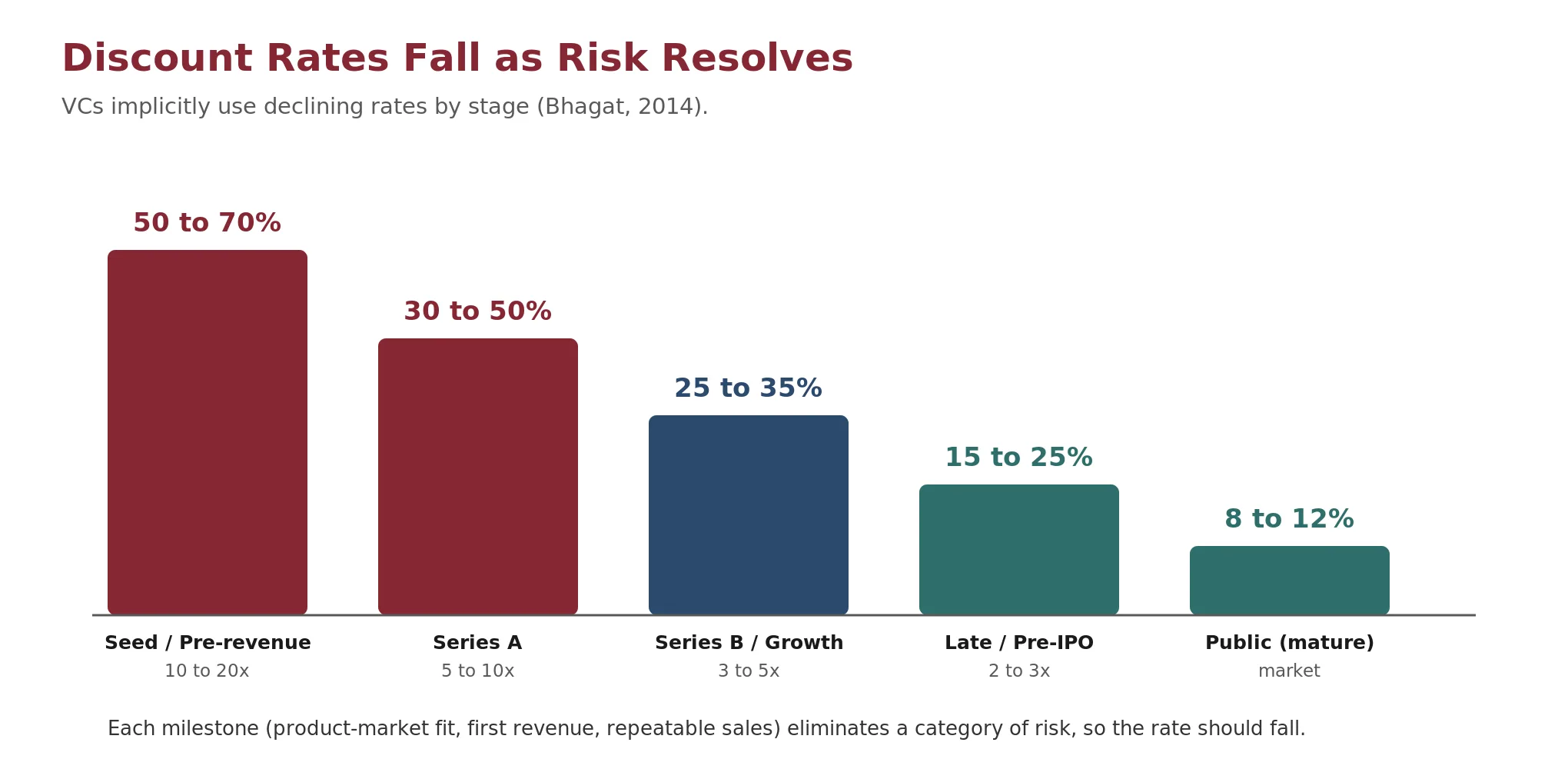
A standard DCF applies a single WACC to every projected year, assuming the business carries the same risk in Year 1 as in Year 10. For mature, stable companies this is a reasonable simplification. For startups and high-growth ventures it is demonstrably false. A pre-revenue startup faces binary risk: will the product work, will customers pay, will the team execute? Each milestone (product-market fit, first revenue, positive unit economics, a repeatable sales process) tends to remove a category of risk for good. A company past $5M ARR with healthy retention is categorically less risky than the same company at $100K ARR, even at the same growth rate. The discount rate should reflect this.
Empirical evidence from Bhagat (2014) shows venture capitalists implicitly use declining discount rates through their target return multiples by stage.
| Stage | Typical discount rate | Implied target multiple |
|---|---|---|
| Seed / pre-revenue | 50 to 70% | 10 to 20x over 5 to 7 years |
| Series A / early revenue | 30 to 50% | 5 to 10x over 4 to 6 years |
| Series B / growth | 25 to 35% | 3 to 5x over 3 to 5 years |
| Late stage / pre-IPO | 15 to 25% | 2 to 3x over 2 to 3 years |
| Public company (mature) | 8 to 12% | market return expectations |
Implementing Year-by-Year Discount Factors
Instead of discounting every cash flow at one WACC, assign a different rate to each year based on the expected risk at that point. The present value of each year's cash flow becomes the cash flow divided by the product of one plus each year's rate.
Formula. PV(CF_n) = CF_n / [(1 + r1)(1 + r2)(1 + r3) ... (1 + rn)]
For a startup expected to be pre-revenue in Year 1 (50%), reach product-market fit in Year 2 (40%), hit $1M ARR in Year 3 (30%), reach $5M ARR in Year 4 (20%), and be acquisition-ready in Year 5 (15%), the cumulative discount factors are 0.667, 0.476, 0.366, 0.305, and 0.265. Compare a flat 30% WACC: the Year 5 factor would be 1 / (1.30)^5 = 0.269, close to the stage-adjusted 0.265, but the Year 1 factors differ sharply (0.667 versus 0.769), reflecting the concentrated risk in the earliest period. Stage adjustment matters most for ventures with high early binary risk, such as biotech and deep tech, and for long forecast horizons, where applying a seed-stage rate to Year 10 makes those cash flows nearly worthless and understates value for a company that will clearly have de-risked. It also gives founders negotiating leverage: if the company has de-risked since the last round, the appropriate rate for the next round should be materially lower.
Check Your Understanding
Knowledge Check 10
Cost of Capital (WACC) & VC Method
As a venture moves from seed toward late stage and clears milestones such as product-market fit and a repeatable sales process, what tends to happen to the discount rate investors apply?
DCF Undervalues Flexibility: Real Options
A discounted-cash-flow value rests on a hidden assumption: that management commits to a single plan today and follows it regardless of what happens next. Real ventures do not behave that way. Founders and investors can expand a promising line, delay a bet until the picture clears, or abandon a plan that is failing. That flexibility has value, and a static DCF omits it, which is one reason a mechanical DCF tends to understate the worth of an early-stage venture.
The intuition splits cleanly in two directions:
- The option to abandon caps the downside. If a project sours, management can stop funding it and walk away, so the loss is bounded rather than open-ended.
- The option to expand captures the upside. If early results are strong, management can pour in more capital and scale, capturing gains a fixed plan would leave on the table.
Formal valuation prices this flexibility with option-pricing methods, generally a binomial lattice or a Black-Scholes framework, treating the decision to continue as a call option on the venture's future value. The mechanics matter less than the core insight: flexibility is worth more when uncertainty is higher. When outcomes are nearly certain, the right to change course is close to worthless because there is little to react to. When the range of outcomes is wide, the ability to expand into good news and abandon bad news is generally where much of the value sits.
Staged Financing Is a Real Option
Venture investors rarely fund an entire plan in one check. Instead they stage capital across rounds, seed, then Series A, then Series B and beyond, with each round tied to milestones the company is expected to hit. This structure is itself a real option. Each round buys the right, not the obligation, to continue. A disappointing milestone lets the investor decline the next round and cap losses, while a strong result justifies a larger follow-on at a higher valuation.
A brief numeric intuition makes the point. Suppose a plan needs $2,000,000 in total.
- Fund it all up front. Committing the full $2,000,000 at once puts the entire amount at risk if the company fails early.
- Stage it. Investing $500,000 now with the remaining $1,500,000 contingent on hitting a defined milestone limits the early loss to $500,000 if the venture stalls, while preserving the upside of continuing if the milestone is met.
The staged path bounds the downside to the money already deployed and keeps the option to scale into good news, which mirrors the abandon-and-expand logic of real options. Staging is not free of tradeoffs. It also imposes discipline on the founders, who must deliver against milestones to unlock further capital, and it shifts the timing of dilution, since later rounds are priced on results the company has since produced rather than on the original plan.
Check Your Understanding
Knowledge Check 11
Valuation & DCF
A venture investor deploys capital across rounds tied to milestones instead of funding the full plan at once. Under high uncertainty, why does this staging add value?
Knowledge Check 12
Valuation & DCF
A static discounted-cash-flow valuation assumes management follows one fixed plan set today. Why does this tend to understate the value of a venture whose managers can expand, delay, or abandon as information arrives?
Part Six
The Market Lens: Comparables and Precedent Transactions
DCF tells you what a business should be worth based on its cash flows. Comparables tell you what the market is currently willing to pay for businesses like it. Both are necessary; neither alone is sufficient.
Trading Comparables
Trading comps value a company by the multiples of publicly traded peers with similar characteristics, assuming similar companies trade at similar multiples, adjusted for growth, profitability, and risk.
- EV to revenue is preferred for high-growth, not-yet-profitable companies, with a typical SaaS range of 5 to 15x forward revenue depending on growth.
- EV to EBITDA is the workhorse for profitable businesses, neutralizing capital structure, tax, and D&A policy, typically 8 to 20x for growth companies and 5 to 10x for mature ones.
- Price to earnings is affected by leverage and less common in venture contexts because earnings are often negative.
- EV to gross profit is emerging for SaaS companies where gross margins vary widely, normalizing for margin differences that distort revenue multiples.
Treat these ranges as current market observations, not fixed constants.
Work the market approach end to end: enter three peer EV/Revenue multiples, the target's revenue, and its net debt. The calculator then takes the median multiple, computes enterprise value, and backs out equity value. Push one peer to an extreme and compare the median against the mean to see why comp selection, not arithmetic, is where the judgment lives.
Precedent Transactions
Precedent transactions analyze multiples paid in completed M&A deals involving similar companies. They differ from trading comps in one critical respect: they include a control premium, typically 20 to 40% above the trading price, that buyers pay for the right to control strategy, capital allocation, and operations. Use precedent transactions when valuing a company for an acquisition, since you are buying control, and trading comps when valuing a minority stake, since you are not.
Check Your Understanding
Knowledge Check 11
Valuation & DCF
You are valuing a company for an acquisition of control. Which comparable set is most appropriate, and why?
Selection Criteria and Pitfalls
The quality of a comparable analysis depends heavily on the quality of the comparable set. Selection should match:
- industry and business model,
- revenue scale,
- growth rate,
- margin profile, and
- geography and end-market.
A $10M revenue company is not comparable to a $500M one, and a 50% grower should not be comped to a 10% grower without adjustment. The critical limitation is that comps tell you what the market pays, not what something is worth. During the 2021 low-rate bubble, SaaS companies traded at 30 to 50x revenue, multiples that reflected euphoria, not intrinsic value. An analyst who used 2021 comps to justify a valuation was anchoring to a distorted market. As a rule of thumb, cross-check comps against a DCF to test whether the implied growth rate is achievable.
The VC Method: Working Backward From Exit
Sahlman (1987) formalized how venture capitalists actually price investments. The VC method is not a DCF: it works backward from a target exit value and applies the investor's required return to derive today's price. It is the dominant framework for pre-revenue and early-revenue companies where traditional DCF inputs, stable cash flows and a reasonable WACC, do not exist.
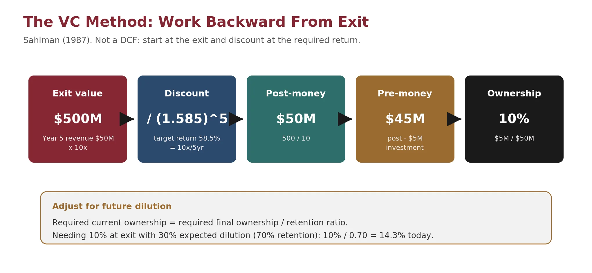
The five steps run as follows. First, estimate terminal value at exit: project revenue or earnings at the expected exit (typically 5 to 7 years) and apply an industry exit multiple, for example projected Year 5 revenue of $50M at a 10x EV to revenue multiple, giving a $500M terminal value. Second, discount to present value at the VC's required return, not WACC: a 10x target in 5 years implies a discount rate of 58.5% per year (10 to the 1/5 power, minus 1). Third, compute post-money: $500M / (1.585)^5 = $500M / 10 = $50M. Fourth, compute pre-money: post-money minus the investment, so $50M - $5M = $45M. Fifth, compute ownership: investment divided by post-money, so $5M / $50M = 10%. The VC needs 10% of the company to achieve their target return, assuming the exit is achieved.
Work backward from the exit: set the exit value, target return, holding period, and investment to derive post-money, pre-money, and required ownership. Then layer in dilution to see the ownership you need to take today. The defaults reproduce the module's walk-through ($500M exit, 58.5% return, 5 years, $5M in → $50M post-money and 10% ownership, rising to 14.3% after 30% dilution).
Check Your Understanding
Knowledge Check 12
Cost of Capital (WACC) & VC Method
Why does the VC method discount at a target return rather than WACC?
Accounting for Future Dilution: The Retention Ratio
The basic method assumes the investor's entry ownership equals their exit ownership. In reality, later rounds, option pool expansions, and anti-dilution provisions reduce ownership before exit. Sophisticated investors adjust with a retention ratio, the fraction of ownership they expect to retain through exit.
Formula. Required Current Ownership = Required Final Ownership / Retention Ratio
If a VC needs 10% at exit and expects 30% cumulative dilution (a 70% retention ratio), they need 10% / 0.70 = 14.3% today, not 10%.
| Component | Formula | Example |
|---|---|---|
| Required final ownership | Investment / (Terminal value / target return) | 10% |
| Expected dilution (future rounds) | Sum of anticipated new shares | about 30% |
| Retention ratio | 1 - expected dilution | 70% |
| Required current ownership | Final ownership / retention ratio | 14.3% |
| Option pool reserve (pre-money) | Typically 10 to 20% at each round | 15% |
| Effective pre-money given away | Investor % + new option pool | 29.3% |
VCs typically require an option pool refresh created before their investment, out of the pre-money, diluting existing shareholders but not the new investor. A 15% pre-money pool means founders give away 15% before the VC's dollars create further dilution. It is a negotiation lever disguised as standard practice: the larger the pre-money pool, the lower the effective pre-money from the founders' perspective. Anti-dilution protection gives current investors extra shares in a down round, full-ratchet or weighted-average, diluting founders further. Participation rights give participating preferred holders their liquidation preference plus a pro-rata share of remaining proceeds, which does not dilute ownership but dilutes the economic value per common share. Pro-rata rights let an investor maintain ownership by investing in future rounds, improving the retention ratio at the cost of more capital.
VCs do not use WACC for three reasons. Portfolio math demands it: if 6 of 10 investments fail completely, the 4 winners need to return the entire fund plus target profit, so a 3x gross fund return requires winners to average 7 to 8x. CAPM inputs generally do not exist for pre-revenue firms: there is rarely an observable beta, a stable capital structure, or a meaningful cost of debt. And the discount rate embeds failure probability implicitly: a 50% required return does not mean the VC expects 50% on each deal, but that across the portfolio, including zeros, the blended return needs to reach the fund's target.
Check Your Understanding
Knowledge Check 13
Cap Tables & Dilution
A VC needs 10% ownership at exit and expects 30% dilution before then. What ownership must they take today?
The Cost Approach: When Assets Define Value
The cost approach values a business at the cost to reproduce or replace its net assets. It is the least common primary method in entrepreneurial finance but serves three roles. As a floor, it sets the minimum value in any negotiation: a company with $10M in net assets is generally not worth less than $10M unless it is burning cash faster than it can be liquidated. For asset-heavy businesses, such as real estate holding companies, equipment leasing, and natural resources, value is in the assets, not operating cash flows. In distressed situations, where cash flows are negative and the going-concern assumption is questionable, the relevant question becomes what the parts are worth separately.
Three methods sit within the cost approach. The adjusted net asset method restates all assets and liabilities to fair market value, not book value, and computes equity as adjusted assets minus adjusted liabilities. Replacement cost asks what it would cost to build the business from scratch today, including physical assets, assembled workforce, customer relationships, and technology, which is useful for IP-heavy companies. Liquidation value asks what a quick, distressed sale would yield, typically 50 to 70% of fair market value for tangible assets and near zero for most intangibles. The approach fails for most startups: a SaaS company with $500K in laptops and servers, $2M in capitalized development, and $50M in annual recurring revenue is worth far more than its asset base suggests. The cost approach captures little of the value in customer relationships, growth trajectory, network effects, or brand. For knowledge businesses it is a necessary floor and rarely the primary valuation.
Valuation Is Not the Same as Deal Economics
A common mistake is treating the stated valuation as the economic reality. The headline valuation, pre-money or post-money, is a starting point, but the actual economics depend on the terms attached to the investment. Two term sheets can offer the same $20M pre-money and produce dramatically different outcomes for founders.
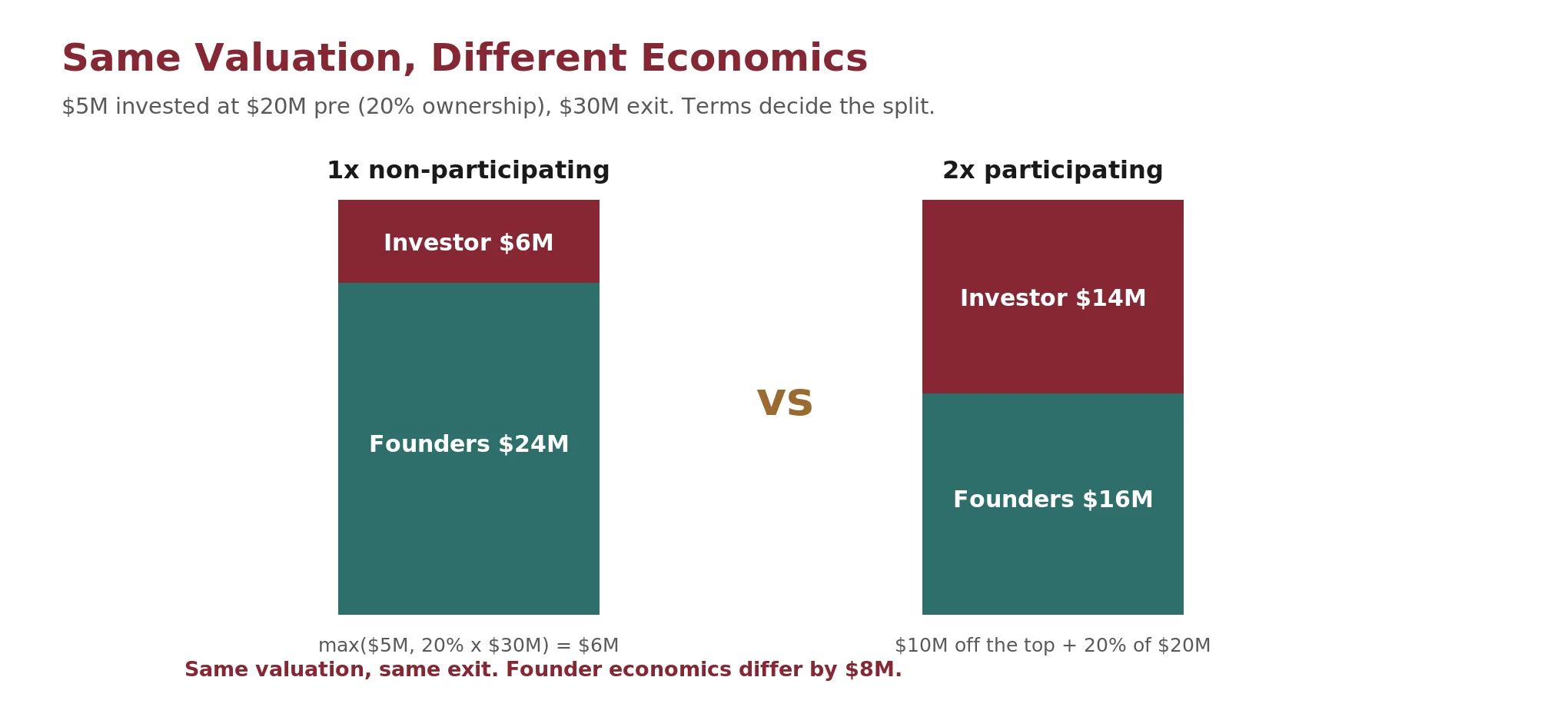
Liquidation preference is the most impactful term. A 1x non-participating preference means the investor gets their money back first, then converts to common. A 2x participating preference means the investor gets 2x their investment back and their pro-rata share of everything remaining. At a $30M exit on a $5M investment at $20M pre (20% ownership), the 1x non-participating investor takes the greater of $5M or 20% of $30M, which is $6M, leaving founders $24M. The 2x participating investor takes $10M off the top, then 20% of the remaining $20M, which is $4M, for a total of $14M, leaving founders $16M. Same valuation, same exit, and founder economics differ by $8M.
Anti-dilution protection reshapes value too. Full-ratchet anti-dilution reprices the entire prior round to the new lower price; weighted-average adjusts proportionally to the size of the down round. In severe down rounds, full-ratchet can transfer 10 to 20% additional ownership from founders to prior investors, making the effective valuation of the original round much lower than stated. An option pool carve-out has a similar effect: a 20% pool created pre-money on a $20M pre means the real pre-money going to existing shareholders is $16M, because $4M is allocated to the unissued pool. VCs negotiate option pools pre-money; founders should push for post-money pools or smaller pools with future refreshes.
Set investment $5M, a 1x preference, 20% ownership, and a $30M exit to reproduce the figure's non-participating case, where the investor takes the greater of $5M or 20% of $30M ($6M) and founders keep $24M.
Check Your Understanding
Knowledge Check 14
Term Sheets & Liquidation Preferences
On a $30M exit, a $5M investor at $20M pre (20%) holds a 2x participating preference. What do founders receive?
Probability-Weighted Scenario Valuation
When future outcomes are uncertain, not merely volatile around a trend, a single-point DCF produces false precision. Probability-weighted scenario analysis models multiple futures, assigns probabilities, and computes an expected value. It is more honest and avoids optimizing around a single forecast that may never materialize. A standard three-scenario structure has a downside (20 to 30% probability, growth stalls or execution falters, value a fraction of the base case), a base case (40 to 50%, the operating plan is achieved), and an upside (20 to 30%, category tailwinds or successful adjacent-market entry, value 1.5 to 3x the base). For early-stage ventures, add a failure scenario (30 to 50% at seed, 15 to 25% at Series A) where value is zero or recovery of remaining cash.
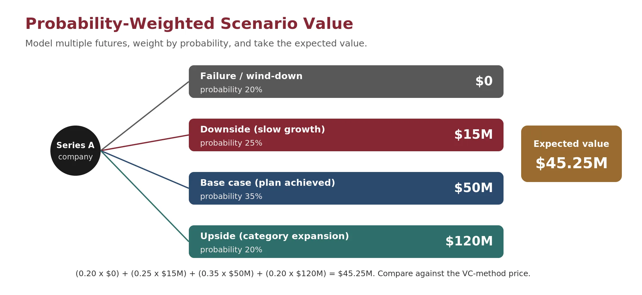
Worked Example: A Series A Expected Value
| Scenario | Probability | Equity value |
|---|---|---|
| Failure / wind-down | 20% | $0 |
| Downside (slow growth) | 25% | $15M |
| Base case (plan achieved) | 35% | $50M |
| Upside (category expansion) | 20% | $120M |
The expected value is (0.20 x $0) + (0.25 x $15M) + (0.35 x $50M) + (0.20 x $120M) = $0 + $3.75M + $17.5M + $24M = $45.25M. This can be compared to a VC-method valuation. If the VC method (at a 40% target return) produces a $40M post-money, the probability-weighted approach suggests the deal is slightly favorable to the investor, paying $40M for a $45.25M expected value. If the VC method produces $60M, the deal may be overpriced relative to the outcome distribution.
Use probability-weighted valuation for binary outcomes, such as biotech drug approval or platform network effects; for wide confidence intervals, when reasonable bull and bear projections differ by 3x or more; as a negotiation tool, since presenting explicit scenarios demonstrates rigor and grounds the discussion in assumptions that can be debated individually; and for board-level capital allocation, where comparing expected values across scenarios beats comparing single-point NPVs.
The defaults reproduce the Series A worked example: failure 20% at $0, downside 25% at $15M, base 35% at $50M, and upside 20% at $120M, for a probability-weighted expected value of $45.25M.
Check Your Understanding
Knowledge Check 15
Valuation & DCF
Scenarios: failure 20% at $0, downside 25% at $15M, base 35% at $50M, upside 20% at $120M. What is the expected value?
Triangulation: No Single Method Is Sufficient
Professional valuators rarely rely on a single method. They compute value several ways and present a range, and the degree of convergence is itself informative. Tight convergence, all methods within 15 to 20%, signals high confidence that the asset is priced consistently regardless of the analytical lens. Wide divergence, methods differing by 50% or more, signals that one or more sets of assumptions is likely wrong, or that the company is in a transitional state where different methods capture different aspects of value.
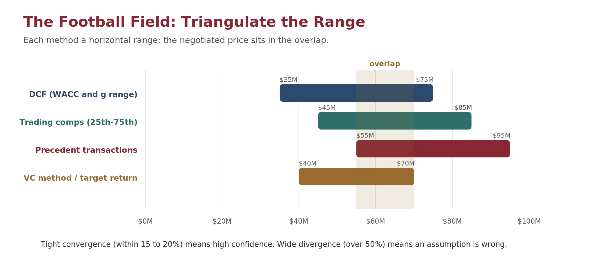
Investment banks present valuations as horizontal bar charts, football fields, showing the range from each method: a DCF range across WACC and terminal-growth assumptions, a trading-comps range from the 25th to 75th percentile, a precedent-transactions range, a VC-method or target-return analysis, and a 52-week trading range if public. The negotiated price almost always falls in the overlap zone where multiple methods agree. If a buyer proposes a price below every method's range, the seller has strong analytical ammunition to push back. If the seller demands a price above every range, they need a compelling strategic rationale to justify the premium.
| Company stage | Primary method | Cross-check with |
|---|---|---|
| Pre-revenue startup | VC method | Replacement cost (floor) |
| Early revenue, high growth | VC method + DCF | Revenue comps |
| Scaling company ($10M+ revenue) | DCF | Trading comps, precedents |
| Mature profitable company | DCF + trading comps | Precedents, asset value |
| Distressed / liquidation | Cost approach | DCF (recovery scenario) |
A method is only as good as its inputs. A DCF with fabricated growth produces a fabricated value; comps with poor comparables produce misleading multiples; the VC method with an unrealistic exit produces a fantasy. The analytical skill is not running the formulas but selecting defensible inputs and pressure-testing them against reality. Before accepting any valuation, ask three questions. What growth rate is implied, and has this company or any comparable ever sustained it? What discount rate was used, and does it reflect the actual risk of this specific business at this specific stage? What exit assumption drives the terminal value, and is there observable evidence, recent transactions or public comps, supporting it? If all three answers are grounded in evidence, the valuation is defensible. If any requires trust me or the market will get there, the valuation is speculation dressed in financial modeling.
Limits of the Toolkit
Each method converts an uncertain future into a present price, and each tends to bury some risks in a single number. The output is only as good as the inputs and the judgment behind them.
The discount rate is the most consequential and least observable input. For private and pre-revenue firms, beta, the equity risk premium, and the market value of equity are estimates, and small errors move value by tens of percent.
Terminal value drives most of a DCF, yet it rests on the least knowable assumptions about the distant future. Present it as a sensitivity range over WACC and g.
The benchmarks and ranges used here, including WACC bands, terminal value of 60 to 80%, 2 to 3% perpetuity growth, a 20 to 40% control premium, a 2 to 6% size premium, and VC target returns by stage, are practitioner heuristics and observed ranges, not laws, and they shift with the market and the cycle.
Time-sensitive figures, including a risk-free rate near 4.3% and Damodaran's implied equity risk premium of 4.23% as of January 2026, will change. Re-source them at the time of any real valuation.
The final discipline is not running the formulas but selecting defensible inputs and pressure-testing them against observable reality. A valuation that requires trust rather than evidence is speculation dressed in financial modeling.