
Week 4CHAPTER 04
Financial Forecasting for Startups
How to build a forecast you can defend, a driver-based, bottom-up approach that connects operating assumptions to cash, runway, and enterprise value. Why a forecast is a structured hypothesis, not a prediction; compound growth and CAGR; trailing-twelve-months, run-rate, and NTM as credibility checks; building revenue from the drivers (volume × price) rather than the outcome; eleven guidelines for a clean model; the revenue engine (sales-headcount and subscription MRR models, market sizing); cash as the constraint (gross vs. net burn, runway, minimum cash, and the financing need); unit economics (margins, CAC, LTV, payback, churn, NRR); pipeline, conversion, and headcount timing; stress-testing with sensitivity, scenario, rolling-forecast, and variance analysis; and the MARCS framework that unifies the whole workflow, with five interactive calculators.
~130 min8 sections50 questions5 tools
Learning objectives (8)
Learning Objectives
By the end of this chapter you should be able to:
- 1Explain why a financial forecast is a structured hypothesis rather than a precise prediction.
- 2Calculate and interpret CAGR, TTM revenue, run-rate revenue, and NTM revenue as tools for evaluating growth and forecast credibility.
- 3Build a driver-based revenue forecast using controllable inputs such as volume, price, sales headcount, productivity ramp, churn, and conversion rates.
- 4Distinguish between outcome-based forecasting and bottom-up forecasting, and explain why bottom-up models are more useful for startup planning.
- 5Construct basic startup cash metrics, including gross burn, net burn, runway, minimum cash balance, and financing need.
- 6Evaluate unit economics using gross margin, contribution margin, CAC, LTV, LTV/CAC, CAC payback, churn, and net revenue retention.
- 7Diagnose forecast risk by using sensitivity analysis, scenario analysis, rolling forecasts, and variance analysis.
- 8Apply the MARCS forecasting framework to clean data, isolate the controllable drivers, build the base case from them, stress-test it against an aspirational stretch overlay, and update the forecast over time.
Part One: A Forecast Is a Structured Hypothesis, and Growth Compounds. Section 1 of 8.
Part One · A Forecast Is a Structured Hypothesis, and Growth Compounds
A Forecast Is a Structured Hypothesis, and Growth Compounds
A Forecast Is a Structured Hypothesis, Not a Prediction
Forecasting is the discipline of using historical data and strategic assumptions to project future states. It converts planning into a rigorous model. In corporate finance, a forecast determines whether a company has the cash to hire, the capacity to expand, or the need to cut costs.
The most important thing to understand is that a forecast is not a prediction of what will happen. It is a structured hypothesis about what could happen, and a framework for responding when reality diverges. The goal is not perfect accuracy; the goal is disciplined preparedness, fast learning, and better decisions as actual results arrive. Accuracy still matters. Forecasts that are consistently wrong without explanation damage credibility with investors, board members, and the team. The discipline is in explaining the variance, learning from it, and improving the next forecast.
This module covers the mechanics: how to build a model from the drivers up, how to stress-test the assumptions, and how to connect the model to the questions founders typically need to answer about cash, runway, and enterprise value. For the line-by-line details of modeling an income statement, Dave Lishego's Founder's Guide to Financial Modeling (2020), a self-published practitioner guide by a venture investment associate, walks through each area with worked examples in Excel. This module focuses on the principles and frameworks that apply regardless of what you are modeling.
Check Your Understanding
Knowledge Check 1
Forecasting & Driver-Based Models
A forecast is best understood as a structured hypothesis rather than a point prediction of what will happen. What is its primary purpose?
Compound Growth Is the Default Trajectory
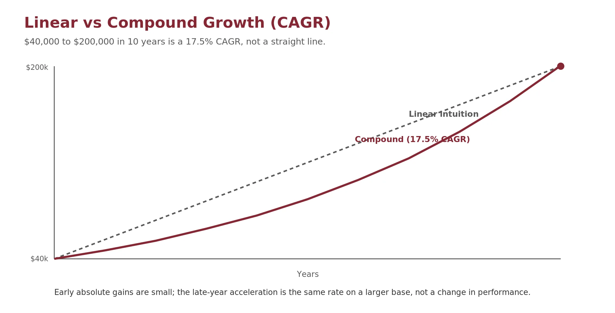
Most people project growth linearly, assuming that if they saved $5,000 this year they will save $5,000 next year. Successful financial trajectories, whether in careers, investments, or business revenue, rarely follow a straight line. They follow a geometric progression. To measure it, analysts use the Compound Annual Growth Rate (CAGR), which smooths the volatility of individual years to reveal the underlying rate required to move from a starting point to an ending point over a period.
Formula. CAGR = (Ending Value / Beginning Value) ^ (1 / n) - 1 where n is the number of years
Worked example: A career trajectory
An entry-level employee earning $40,000 aims to earn $200,000 within 10 years. They are not looking for linear raises. They are solving for a CAGR of about 17.5%: ($200,000 / $40,000) to the 1/10 power is 5 to the 0.1 power, which is about 1.175, minus 1. Consistent annual raises of roughly 17.5% are required to hit the target.
Understanding CAGR changes how you view the early years of any growth curve. On a compound curve, the absolute dollar growth in the early years is small even when the percentage growth is high. The vertical acceleration in later years is not a change in performance; it is the same rate applied to a larger base. This is true for salaries, for startup revenue, and for investment returns.
Adjust the beginning value, target, and horizon to see the CAGR. The defaults reproduce the worked example above.
Interactive Tool
Compound Growth (CAGR)
CAGR
17.5%
constant annual rate
Total growth
5.0×
end ÷ begin
First-year gain
$6,985
same rate, small base
Final-year gain
$29,732
same rate, larger base
The late-year acceleration is not better performance, it is the same 17.5% rate on a larger base. Straight-line intuition would add about $16,000 every year; compounding back-loads the dollars.
Check Your Understanding
Knowledge Check 2
Forecasting & Driver-Based Models
An employee earning $40,000 wants to reach $200,000 in 10 years. What constant annual growth rate would they need to sustain?
Trailing Twelve Months and Forecast Credibility
Trailing Twelve Months, or TTM, measures the most recent 12 consecutive months of a financial metric, regardless of fiscal year-end. It is commonly used for revenue, EBITDA, net income, and other valuation or diligence metrics. The standard formula starts with the last full fiscal year, adds the most recent current-year activity, and removes the overlapping prior-year period.
Formula. TTM = Last Full Fiscal Year + Current Year-to-Date - Prior-Year Same-Period Year-to-Date
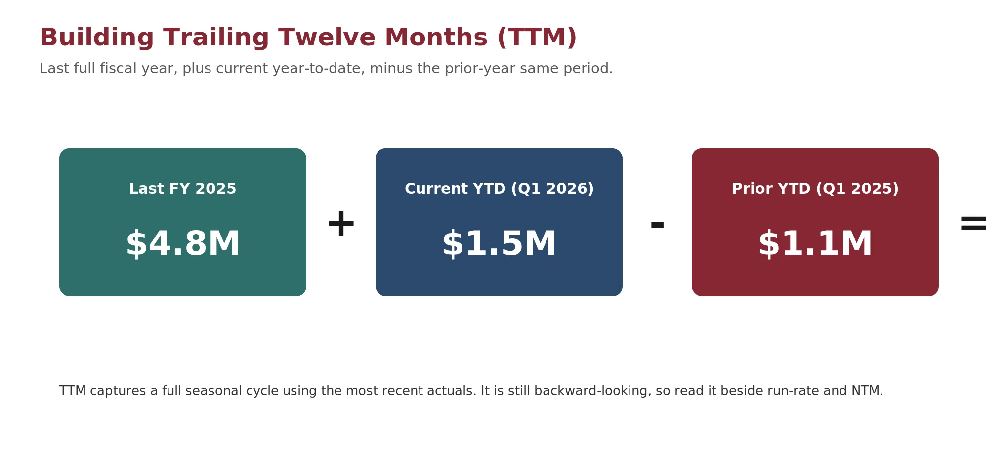
For example, with FY2025 revenue of $4.8 million, Q1 2026 revenue of $1.5 million, and Q1 2025 revenue of $1.1 million, TTM revenue is $4.8 million + $1.5 million - $1.1 million = $5.2 million. TTM captures a full twelve-month period using the most recent results, so it is usually more relevant than the last fiscal year alone. It also avoids simple annualization: multiplying a single quarter by four would overstate a seasonally strong quarter or understate a weak one, while TTM spans a full seasonal cycle. TTM and LTM (Last Twelve Months) are used interchangeably; TTM is more common in public-company reporting, LTM in private-company diligence.
Investors often use TTM as the denominator in valuation multiples such as EV to TTM revenue, EV to TTM EBITDA, and price to TTM earnings, because the last fiscal year may be stale by the time a transaction closes. TTM is still backward-looking. For a fast-growing company it may understate the current trajectory; for a declining company it may overstate performance. Compare it against other measures rather than using it in isolation.
Check Your Understanding
Knowledge Check 3
Financial Statements & Cash Flow
FY2025 revenue was $4.8M, Q1 2026 was $1.5M, and Q1 2025 was $1.1M. What is TTM revenue?
TTM Is an Analytical Choice, Not an Automatic Answer
The measurement window matters. A standard TTM period works well for stable or steadily growing businesses but can mislead after an inflection. If the company lost its largest customer five months ago, TTM still includes seven months of that revenue, flattering the run rate. If it signed a major contract two months ago, TTM includes ten months before that contract existed, understating the trajectory. Diligence teams run multiple views side by side.
| Metric | What it shows | Main risk |
|---|---|---|
| TTM / LTM | Most recent 12 months of actual performance | May include stale revenue or miss recent inflections |
| Run-rate revenue | Most recent month or quarter annualized | Overstates if seasonality or one-time spikes exist |
| NTM | Next 12 months from forecast or consensus | Depends heavily on management assumptions |
| L6M annualized | Last six months annualized | More current, but may ignore seasonality |
| TTM-3 | TTM ending three months before the latest period | Checks recent window dressing, but less current |
The best analysis does not ask which number is correct. It asks what each number tells us. TTM shows where the business has been, run-rate where it appears to be today, and NTM where management believes it is going. The spread between them often tells you more about forecast risk than any single metric. If NTM is three times TTM and run-rate depends on a recent spike, investors are being asked to underwrite an inflection that has not yet been proven.
Check Your Understanding
Knowledge Check 4
Forecasting & Driver-Based Models
In a diligence review, forward-looking next-twelve-month (NTM) revenue is three times trailing-twelve-month (TTM) revenue, and the annualized run-rate rests on a recent one-time spike. What does the spread between these three views signal?
Build From the Drivers, Not the Outcome
A common error is to predict the outcome rather than the inputs. Stating that revenue will be $100,000 is a guess. A defensible model uses driver-based forecasting, which breaks a goal into its component variables. In its simplest form, revenue is a function of two controllable drivers: volume (the quantity of units sold, hours worked, or projects completed) and price (the rate per hour, cost per unit, or contract value).
Formula. Revenue = Volume x Price
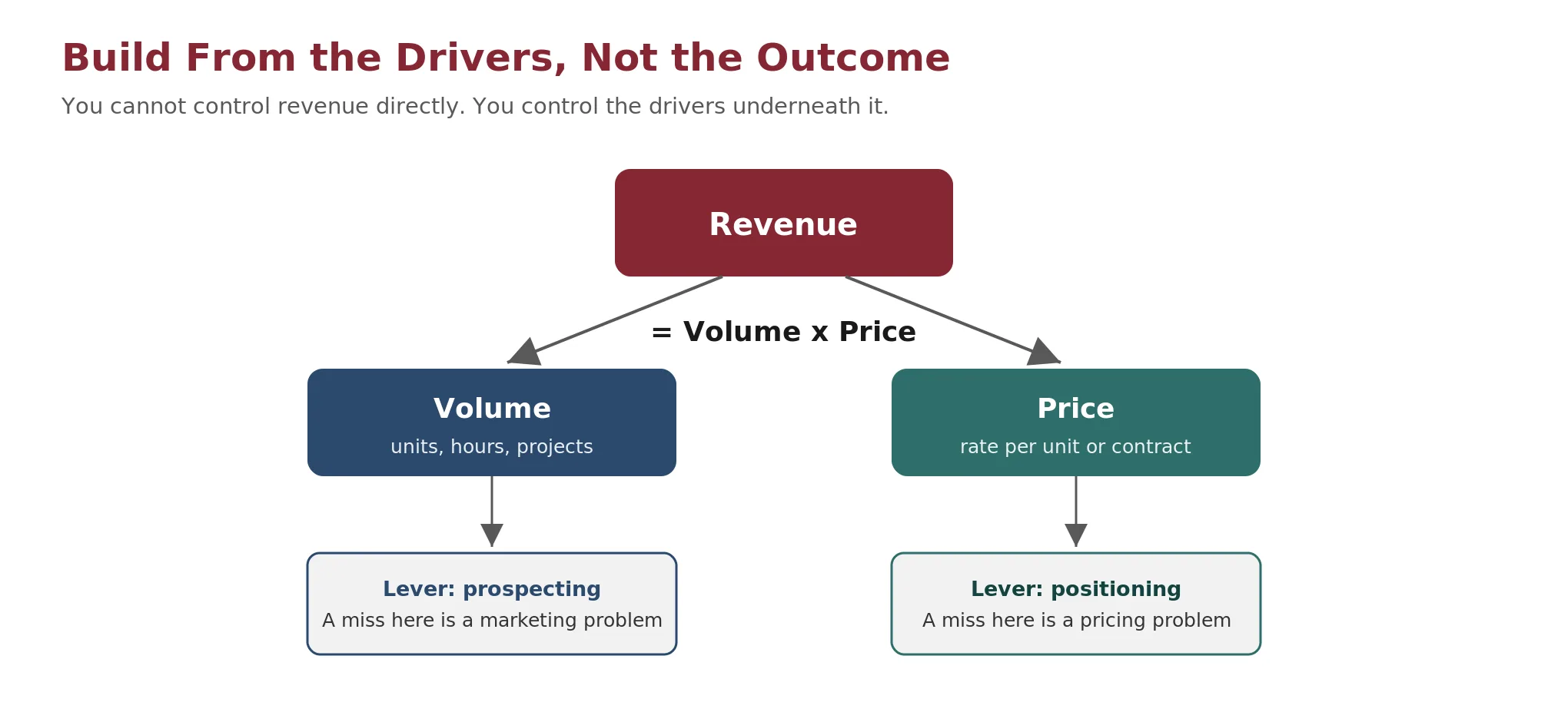
By forecasting the drivers, you gain operational clarity. You do not directly control revenue, but you can influence volume through prospecting and price through skills and positioning. When a forecast is missed, a driver-based model reveals the root cause. A miss from low volume calls for a marketing solution; a miss from low price calls for a positioning or negotiation solution.
Worked Example: A Three-Year Consultant Forecast
A freelance consultant models the drivers rather than guessing at total income.
| Driver | Year 1 | Year 2 | Year 3 |
|---|---|---|---|
| Billable hours / month | 80 | 90 | 100 |
| Hourly rate | $75 | $85 | $100 |
| Months worked | 11 | 11 | 11 |
| Annual gross revenue | $66,000 | $84,150 | $110,000 |
| Growth rate (YoY) | - | +27.5% | +30.7% |
The forecast is not 'I will make $110,000 in Year 3.' It is 'I will work 100 billable hours per month at $100 per hour for 11 months,' which is $110,000. The latter is actionable; the former is wishful thinking. Each figure ties to a driver the consultant can influence.
Check Your Understanding
Knowledge Check 5
Forecasting & Driver-Based Models
A founder writes 'Revenue will be $100,000' with no supporting detail. Why is this statement better described as a guess than a forecast?
Eleven Guidelines for Building a Financial Model
Building a model is more art than science, and there is rarely one right answer. The following guidelines, adapted from Lishego (2020) as practitioner consensus rather than empirical findings, describe what investors and CFOs expect a well-built model to look like.
- Build your model in Excel. Spreadsheets let anyone audit the logic, trace formulas, and modify assumptions. Excel is the professional standard for investor-facing models.
- Build a cash flow model. Revenue does not equal cash. A company can be profitable on paper and run out of money. The income statement shows viability; the cash flow model shows survival.
- Look ahead 3 to 5 years. Seed investors typically want three years, Series A and beyond up to five. The further out, the less precise, but the exercise forces you to think about the trajectory.
- Build monthly, summarize annually. Monthly granularity is essential for managing cash, tracking variance, and spotting seasonality. Annual summaries communicate the big picture.
- Build from the bottom up. Top-down 'we will capture X% of the market' assumptions are not operating plans. Build from the activities that generate revenue: reps, units per rep, price per unit.
- Code and label assumptions dynamically. Every input belongs in a dedicated assumptions section, not hard-coded into formulas, so one change flows through the whole model.
- Document assumptions with sources. Note where each input came from: customer conversations, market research, benchmarks, or prior operating data. This provides credibility.
- Balance detail and simplicity. A model with 200 line items is not better than one with 40 if the detail does not change the conclusions. Model what is material; aggregate the rest.
- Focus on expenses. Founders obsess over revenue, but expenses are more predictable and controllable. Precise expenses with conservative revenue is more credible than the reverse.
- Build the base case from evidence. The base case is the most evidence-based operating plan, neither optimistic nor pessimistic. Then build a downside case and reserve the upside for favorable execution.
- Make it user-friendly. Color-code inputs versus calculations, format consistently, and label every row. The model will be read by people who did not build it.
Check Your Understanding
Knowledge Check 6
Forecasting & Driver-Based Models
Why is building a cash flow model, alongside an income statement, treated as essential in a startup financial model?
Part Four
Revenue Forecasting: The Engine of the Model
Revenue is where most founders start and the line investors scrutinize most closely. The customer acquisition model drives the number of units sold, and the pricing model dictates revenue per unit. Because the acquisition model also shapes the overall structure of the financial model, it is the right place to begin. Revenue equals units sold times price per unit, and the critical question for a startup is where the units come from. The two patterns below, from Lishego (2020), each build from the bottom up.
The Sales Team Headcount Model
For a direct sales motion, revenue is driven by the number of productive reps and the units each closes. The model starts with a hiring plan: each rep has a start date, and a new hire is not immediately productive. A time-to-productivity assumption, typically 60 to 90 days, accounts for ramp. Sales headcount counts reps whose hire date is before month-end; productive reps count those whose hire date plus ramp is before month-end; and units sold equals productive reps times units per productive rep.
| Jan 2019 | Feb 2019 | Mar 2019 | Apr 2019 | |
|---|---|---|---|---|
| Sales headcount | 1 | 1 | 1 | 2 |
| Productive reps | 1 | 1 | 1 | 1 |
| Units sold (2 per rep) | 2 | 2 | 2 | 2 |
Assumptions: three reps starting Sep 2018, Apr 2019, and Jul 2019, a 90-day ramp, and 2 units per productive rep per month. The model is powerful because every assumption is testable. If revenue is below plan, you can diagnose whether the problem is headcount, ramp time, or quota attainment, and each diagnosis leads to a different operational response.
Check Your Understanding
Knowledge Check 7
Forecasting & Driver-Based Models
In a headcount-driven sales model, a rep is hired in January with a 90-day time to productivity. When does the model first credit that rep with sales?
The Subscription MRR Model
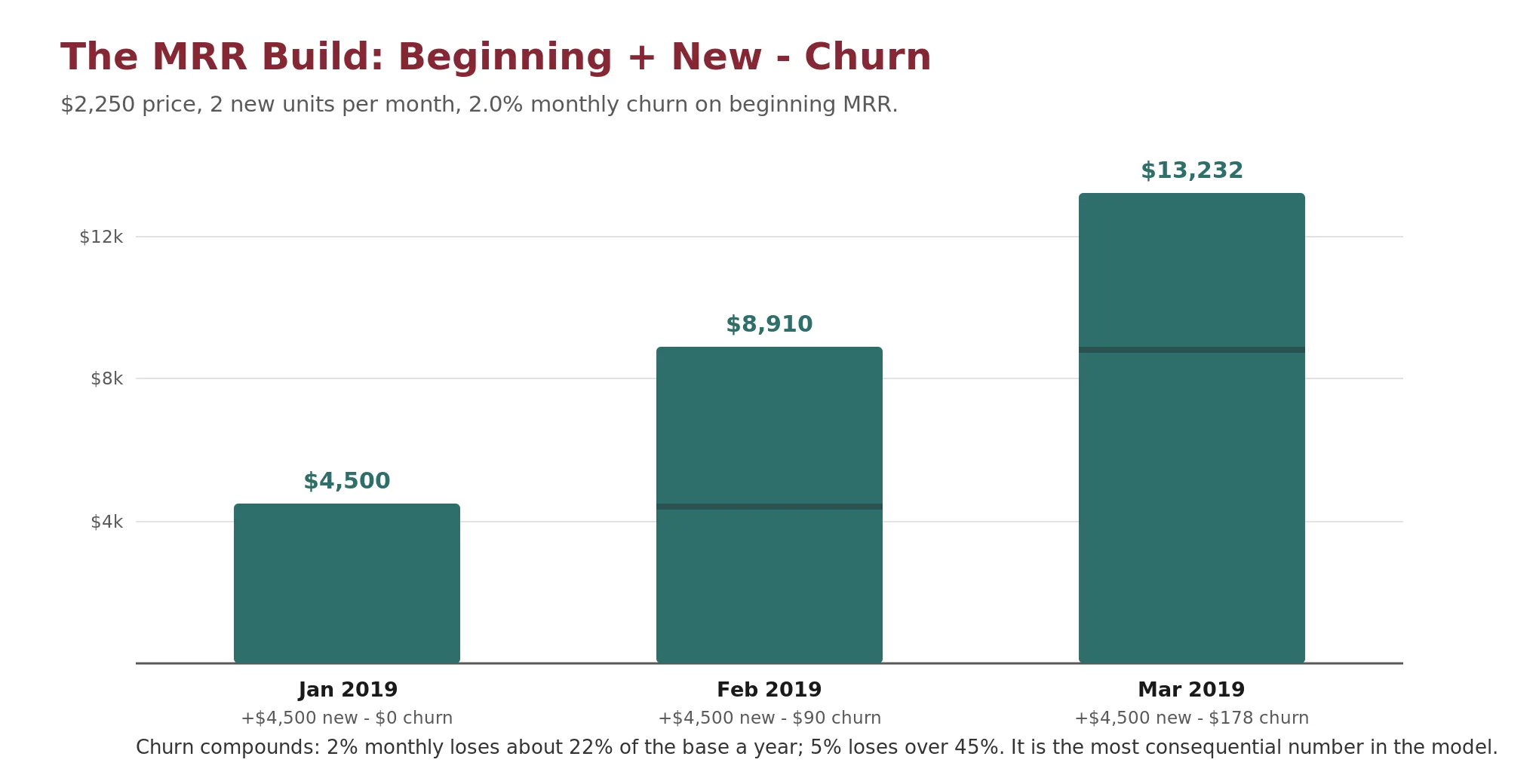
For subscription businesses, revenue depends not only on new subscribers each month but on the cumulative base retained. Lishego (2020) recommends modeling Monthly Recurring Revenue: ending MRR equals beginning MRR (prior month's ending), plus new MRR (new subscribers times price), minus churn MRR (monthly churn rate times beginning MRR).
Formula. Ending MRR = Beginning MRR + New MRR - Churn MRR
Worked example: a three-month MRR build
Assumptions: $2,250 price per month, 2 new units per month ($4,500 new MRR), and 2.0% monthly churn applied to beginning MRR.
| Jan 2019 | Feb 2019 | Mar 2019 | |
|---|---|---|---|
| Beginning MRR | $0 | $4,500 | $8,910 |
| New MRR | $4,500 | $4,500 | $4,500 |
| Churn MRR (2.0%) | $0 | ($90) | ($178) |
| Ending MRR | $4,500 | $8,910 | $13,232 |
The churn assumption is the most consequential number in a subscription model. A company with 2% monthly churn loses roughly 22% of its base annually; at 5% it loses over 45%. Small changes in churn compound dramatically over a multi-year forecast, which is why investors spend disproportionate time on retention.
Adjust the price, new units per month, and monthly churn rate to build the MRR curve. The defaults reproduce the three-month worked example above ($4,500 → $8,910 → $13,232).
Check Your Understanding
Knowledge Check 8
Forecasting & Driver-Based Models
A subscription business has 2% monthly churn. Roughly how much of its base does it lose in a year?
Market Size Frames the Opportunity but Does Not Drive the Forecast
Market size should not be the primary revenue driver in a startup forecast, but it serves as an external constraint and reasonableness check. A top-down 'we will achieve X% market share by year Y' is not an operating plan: it does not help you hire, does not tell you when to raise, and does not reveal which assumptions are fragile. TAM, SAM, and SOM still matter for framing venture scale and evaluating go-to-market credibility. Market size belongs in the pitch and the strategic framing, not in the cells of the revenue model. Use it as a sanity check: if projected revenue reaches an unrealistic share of the market, revisit the assumptions.
The Same Logic Applies to Every Line Item
The driver-based approach applies equally to cost of goods sold, operating expenses, and headcount. Model COGS as a percentage of revenue (the gross margin assumption) or from component costs like hosting, support salaries, and payment fees; at an 80% gross margin, COGS equals revenue times 20%. Model headcount by function with start dates and fully loaded costs, the same logic as the sales team model. The key principle is consistency: if you model revenue from the bottom up, model expenses from the bottom up. A model that projects revenue from a detailed sales plan but plugs SG&A as a flat monthly number signals that the founder has not thought carefully about the cost structure.
Cash Is the Constraint: Burn, Runway, and the Financing Need
For a pre-revenue or early-revenue startup, cash management is the primary financial discipline. Three metrics define the cash position. Gross burn is total monthly cash outflows: payroll, rent, hosting, marketing, everything. Net burn is outflows minus inflows: a company spending $150,000 and collecting $50,000 has a $100,000 net burn.
Formula. Net Burn = Total Monthly Cash Outflows - Total Monthly Cash Inflows
Formula. Runway (months) = Current Cash / Monthly Net Burn
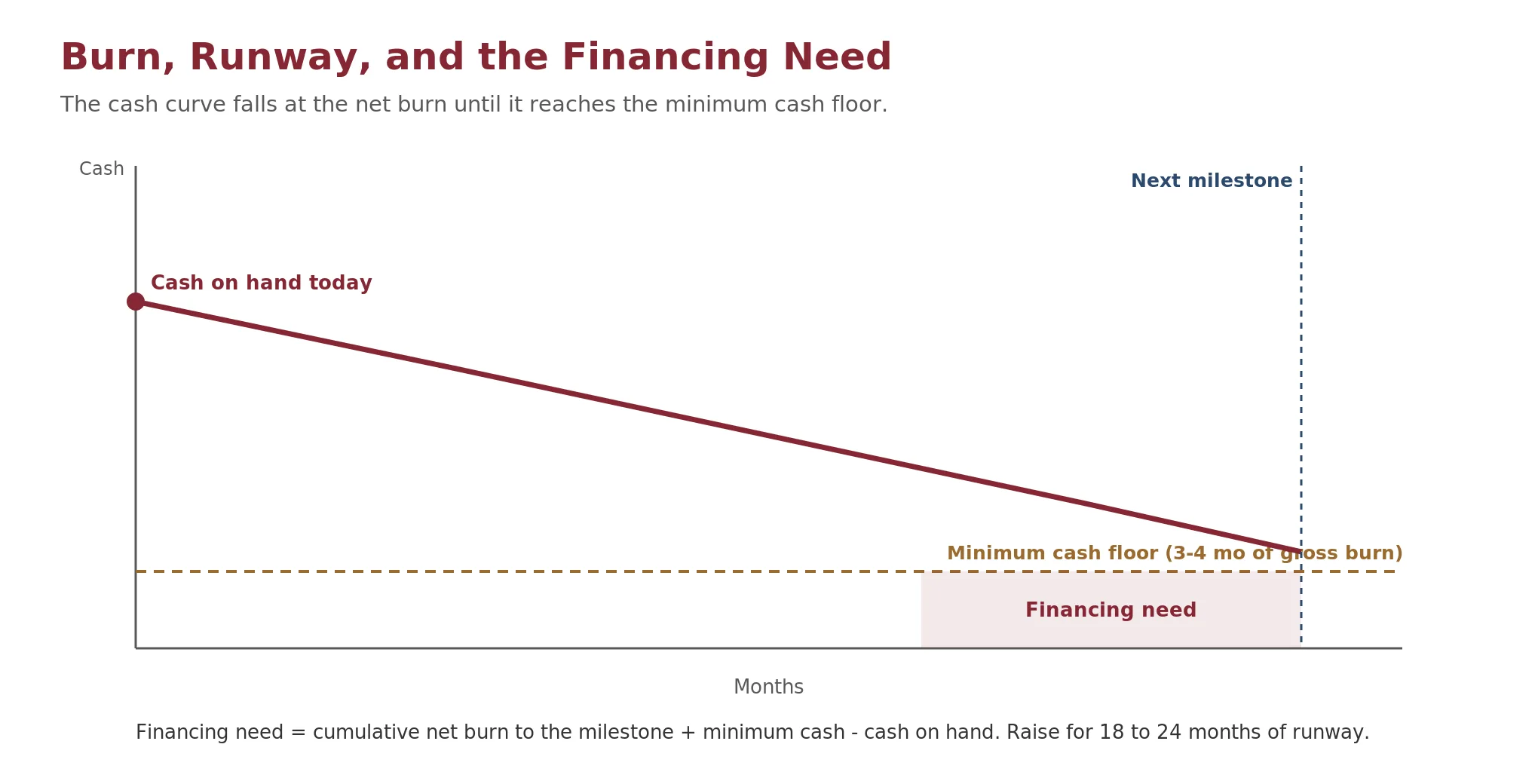
Runway is the number of months the company can operate before it runs out of cash. A company with $1.2 million and a $100,000 net burn has 12 months; the same company at $150,000 net burn has 8. In practice burn changes as the company hires and grows, so the model should compute runway dynamically. A general guideline: raise enough to fund 18 to 24 months of runway, because the next fundraise itself takes 3 to 6 months, and running a raise with under 6 months of runway leaves the founder in a weak position.
Check Your Understanding
Knowledge Check 9
Runway, Burn & Financing Need
A startup holds $900,000 in cash and burns $150,000 net per month. What is its runway?
Sizing the Raise: Minimum Cash and the Financing Need
The model should include a minimum cash balance, the floor beneath which operating becomes risky, commonly 3 to 4 months of gross burn. The financing need then tells the founder how much to raise. It is among the most important outputs for a company that is not yet cash-flow positive.
Formula. Financing Need = Cumulative Net Burn Through Target Milestone + Minimum Cash Balance - Cash on Hand
WORKED EXAMPLE: SIZING THE RAISE
Suppose cumulative net burn to the next milestone is $1.8 million, the minimum cash balance is $0.45 million (about 3 months of gross burn), and cash on hand is $0.8 million. The financing need is $1.8 million + $0.45 million - $0.8 million = $1.45 million. That is the amount to raise to reach the milestone with a safe cash floor intact.
Adjust the monthly net burn, months to the milestone, minimum cash balance, and cash on hand to size the raise. The defaults reproduce a representative case ($0.15M per month burn over 12 months = $1.8M cumulative net burn, $0.45M minimum cash, $0.8M on hand, yielding a $1.45M financing need).
Check Your Understanding
Knowledge Check 10
Runway, Burn & Financing Need
Cumulative net burn to the milestone is $2.4M, minimum cash is $0.6M, and cash on hand is $1.1M. What is the financing need?
The Three Statements Articulate
A forecast that tracks cash without tracking profit, or profit without tracking cash, tends to mislead. The three financial statements articulate, meaning they lock together, and each one measures something the others do not.
- The income statement records accrual profit for the period. Revenue is booked when it is earned and expenses when they are incurred, regardless of when cash actually moves.
- Net income does not disappear at period end. It closes into retained earnings on the balance sheet, which is how a profitable period adds to equity and a loss erodes it.
- The cash flow statement reconciles accrual net income to the actual change in cash. It adds back non-cash charges such as depreciation, adjusts for changes in working capital (receivables, inventory, and payables), and layers in the investing and financing flows.
- The balance sheet must balance because every flow lands in two places. A dollar of depreciation, for instance, reduces net income and reduces the carrying value of the asset at the same time.
For a founder this is not bookkeeping trivia. Profit on the income statement is not cash in the bank. A company can report positive net income while its cash falls, because receivables are growing, inventory is building, or capital is being spent. Only the linked model, with all three statements wired together, shows when the company actually runs out of money.
A Minimal Linked Model
A single-period example shows the wiring. Every number below flows into the next statement, and the balance sheet check confirms the model is internally consistent.
Income statement for the period. Revenue 1,000; COGS 400; gross profit 600; operating expenses 500 (including 100 of depreciation); EBIT 100. With no interest or tax, net income is 100.
Cash flow statement (indirect method). Start from net income 100. Add back depreciation 100. Subtract the increase in accounts receivable 50. Subtract the increase in inventory 30. Add the increase in accounts payable 20. Cash from operations is 140. Investing: capital expenditure (200), so cash from investing is (200). Financing: equity raised 300, so cash from financing is 300.
Formula. Net Change in Cash = 140 - 200 + 300 = 240
Balance sheet articulation (period change). On the asset side: cash +240; accounts receivable +50; inventory +30; property, plant and equipment +100 (that is 200 of capex minus 100 of depreciation). Total asset change is +420. On the other side: accounts payable +20; paid-in capital +300; retained earnings +100 (equal to net income). Total liabilities-plus-equity change is +420. The two sides agree, which is the built-in check that the model is internally consistent.
The takeaway: the company earned 100 of accrual profit yet its cash rose by 240 only because it raised 300 of equity. Operations plus investing alone drained cash, since 140 - 200 is negative 60.
Check Your Understanding
Knowledge Check 15
Financial Statements & Cash Flow
A company reports positive net income for a period and pays no dividends. Where does that net income land on the balance sheet?
Knowledge Check 16
Financial Statements & Cash Flow
A company reports net income of 100. In the same period it adds back 100 of depreciation, receivables rise 50, inventory rises 30, payables rise 20, it spends 200 on capital expenditure, and it raises 300 of equity, so cash rises 240. What best explains why cash rose 240 while net income was only 100?
Five Questions a Founder Forecast Should Answer
A model is not an academic exercise. For a founder, it exists to answer specific questions. A forecast that leaves these five unanswered is generally incomplete.
- How much cash do we need? The forecast should produce a clear financing need from the cash flow model, not the income statement.
- How long is our runway? Given current cash and net burn, how many months before the company runs out? This is among the most important numbers in early-stage finance.
- What milestones can we reach before the next raise? Investors generally fund milestones, not time. Show what the company achieves within the current cash window.
- What assumptions need to hold for this business to work? Make conversion, churn, contract value, and sales cycle explicit.
- Which drivers create or destroy enterprise value? Some assumptions move valuation dramatically; the model should reveal which inputs have the highest leverage.
Part Six
Unit Economics Drive Enterprise Value
Unit economics describe the fundamental profitability of a single customer or transaction. They answer whether the business makes money at the unit level, independent of scale. A company can grow revenue rapidly and still destroy value if the unit economics do not work.
Gross Margin and Contribution Margin
Gross margin is the share of revenue remaining after the direct costs of delivery. SaaS gross margins of 70 to 85% are typical; marketplaces run 30 to 50%. Contribution margin goes further, subtracting all variable costs to acquire and serve a customer, including sales commissions, onboarding, and variable support. If contribution margin is negative, the company loses money on every customer regardless of volume, and growth accelerates the losses. That is a business-model problem, not a scale problem.
Formula. Gross Margin % = (Revenue - COGS) / Revenue
Formula. Contribution Margin = Revenue per Customer - All Variable Costs per Customer
CAC, LTV, and the Ratio That Matters
Customer acquisition cost measures the total cost of acquiring one new customer, including marketing, sales salaries and commissions, and tools. It is most useful segmented by channel and customer type, because blended CAC can hide one efficient channel and one that is hemorrhaging money. Lifetime value estimates the total value a customer generates over the relationship.
Formula. CAC = Total Sales and Marketing Spend / New Customers Acquired
Formula. LTV = ARPU per Month / Monthly Churn Rate
Formula. ARPU (Average Revenue Per User) is calculated by dividing your total revenue by the total number of active users over a specific period (such as a month or a year).
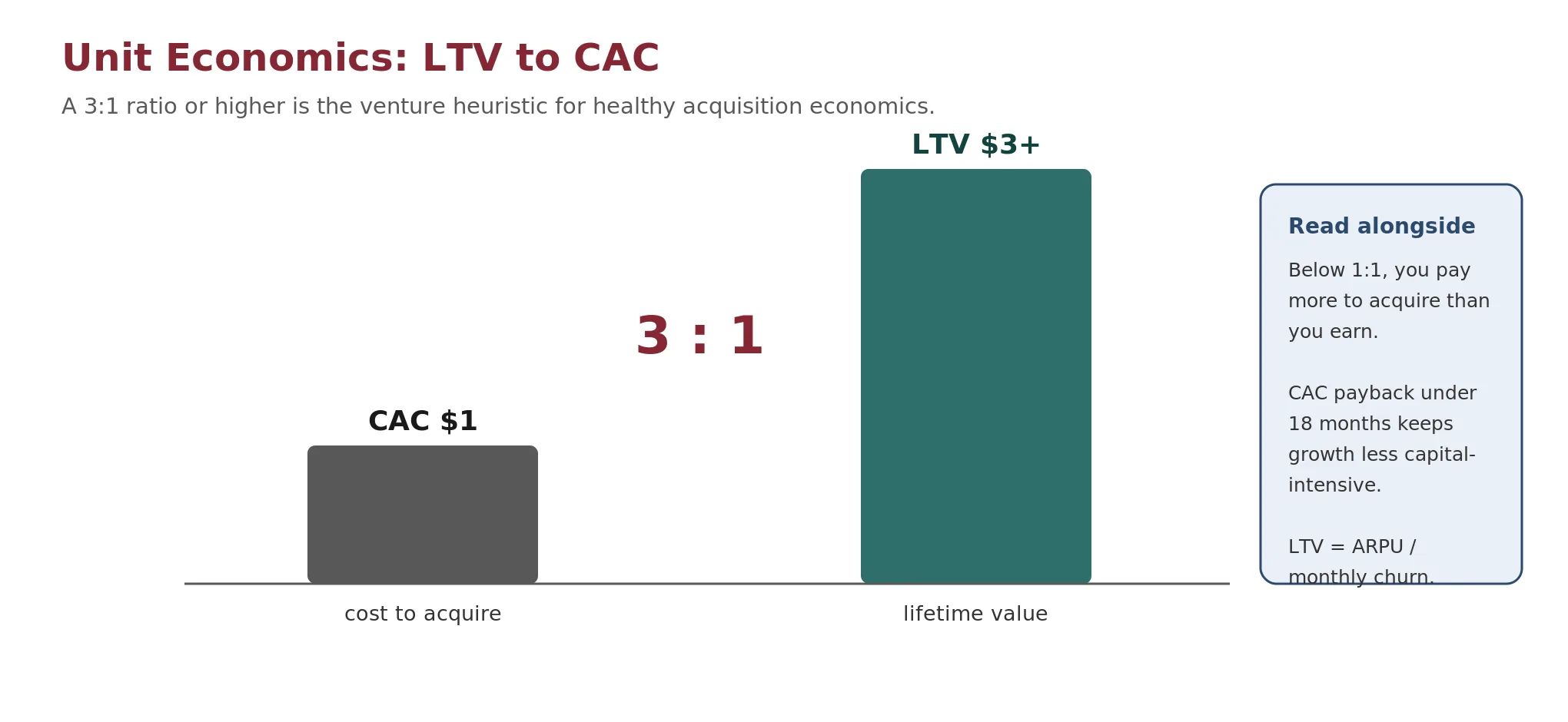
A conservative LTV uses gross profit rather than revenue: (ARPU times gross margin) divided by monthly churn. The LTV to CAC ratio is among the most-watched metrics in venture capital. A ratio of 3 to 1 or higher is the heuristic for healthy economics, meaning at least $3 of lifetime value for every $1 of acquisition cost. Below 1 to 1, the company pays more to acquire customers than it earns from them. Treat these thresholds as conventions, not measured constants.
LTV to CAC tells you whether the economics are profitable; CAC payback tells you how long it takes to recover the investment. A 12-month payback means funding a year of acquisition cost before the customer turns profitable, which directly affects cash and runway. For most SaaS businesses, a payback under 18 months is the benchmark.
Formula. CAC Payback (months) = CAC / (Monthly Revenue per Customer x Gross Margin %)
Enter revenue per customer, gross margin, monthly churn, acquisition spend, and new customers per month. The calculator then computes CAC, LTV, the LTV to CAC ratio, and CAC payback, where a 3 to 1 ratio and a payback under 18 months are the venture heuristics for healthy economics.
Check Your Understanding
Knowledge Check 11
Unit Economics & LTV/CAC
A SaaS product earns $200 ARPU per month at 2% monthly churn. What is the revenue-basis LTV?
Churn and Net Revenue Retention
Churn is the most powerful lever in a subscription business. Logo churn is the percentage of customers who cancel; revenue churn is the percentage of MRR lost to cancellations and downgrades, which can differ when customers have different contract values. Net revenue retention is the percentage of revenue kept from existing customers after churn, downgrades, and expansion. Above 100% means the company grows even without acquiring new customers, the most efficient form of growth because it requires no incremental acquisition cost. Top SaaS companies reach 110 to 130%.
Formula. NRR = (Beginning MRR + Expansion MRR - Churn MRR - Downgrade MRR) / Beginning MRR
Check Your Understanding
Knowledge Check 12
Unit Economics & LTV/CAC
A company reports net revenue retention above 100%. What does that indicate?
Pipeline, Conversion, and Headcount Timing
The revenue model is only as good as the assumptions feeding it. For a sales-driven go-to-market, three metrics connect the model to operational reality. The sales cycle is the average number of days from first contact to closed deal. Enterprise cycles of 60 to 90 days or longer mean a rep hired in January will not close a first deal until March or April at the earliest. The forecast must account for this lag, or revenue projections will be front-loaded relative to reality.
Pipeline conversion is the percentage of qualified opportunities that convert to closed deals. If a team generates 100 qualified opportunities per quarter and closes 25, conversion is 25%. Working backward from a revenue target, conversion determines how many opportunities the team must generate, which sets the marketing spend and SDR headcount required.
Formula. Required Opportunities = Revenue Target / (Average Deal Size x Pipeline Conversion Rate)
For example, to add $1.0 million in new revenue with an average deal of $50,000 and 25% conversion, the team needs $1,000,000 divided by ($50,000 times 25%, which is $12,500), or 80 qualified opportunities.
Headcount timing
Hiring is the largest expense for most startups, and the timing of hires is the largest source of expense variance. Three timing factors matter:
- time to hire (the lag from opening a role to a start date, 30 to 60 days for most roles)
- time to productivity (the ramp before a hire is fully effective, 60 to 90 days for sales reps)
- fully loaded cost (salary plus benefits, taxes, equipment, and recruiting, commonly 1.25 to 1.4 times base salary)
Each hire should appear as a line with a start date and a fully loaded monthly cost. The expense hits the profit and loss on the start date, but revenue is delayed by the ramp. That mismatch is one of the main reasons startups need external capital.
Enter a revenue target, average deal size, and conversion rate to see the required opportunities and the pipeline coverage needed. The default values reproduce a $1.0M target with a $50k deal and 25% conversion, which yields 80 opportunities and $4.0M of pipeline.
Stress-Test, Roll Forward, and Close the Loop
A forecast represents a single path, the base case. Since we are predicting the future, drawing conclusions from one scenario tends to invite surprises, and the longer the horizon, the more likely they become. Professional models use two stress-testing techniques before committing to a plan.
Sensitivity analysis isolates a single variable to measure its impact: if only monthly churn rises from 2% to 4%, what happens to Year 3 ending MRR? If ramp extends from 90 to 120 days, what happens to quarterly revenue? The purpose is to identify single points of failure and reveal which assumptions matter most. If a 1% change in churn breaks the model, churn is the critical variable and warrants the most rigorous forecasting.
Scenario analysis changes multiple variables at once to simulate a distinct narrative. The standard set is a bull case (high growth, favorable conditions, revenue above plan and expenses below), a base case (the most evidence-based operating plan), and a bear case (contraction: sales cycles lengthen, churn rises, a key hire fails, and costs run ahead of plan).
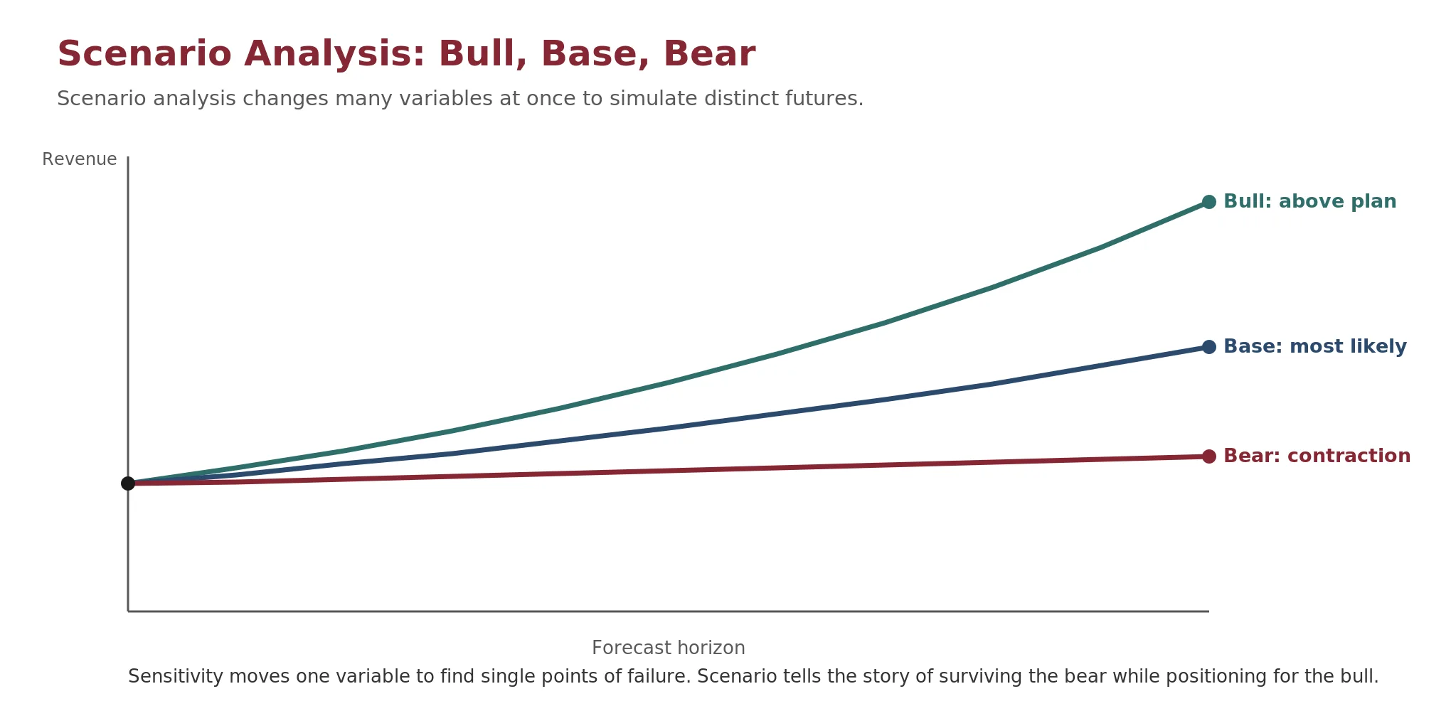
Strong analysts provide both. The most robust plans survive the bear case while positioning for the bull. For a founder, the bear case answers the question most investors ask silently: what happens if this does not work?
Check Your Understanding
Knowledge Check 13
Forecasting & Driver-Based Models
What distinguishes sensitivity analysis from scenario analysis?
Rolling Forecasts Keep the Model Alive
Traditional budgeting sets a static annual plan, then measures against a fixed baseline that reality rarely respects. A rolling forecast continuously extends the horizon: rather than forecasting the next calendar year, you forecast the next 12 months on a rolling basis, regardless of where you are in the fiscal year. Every month, drop the completed month and add a new one to the end.
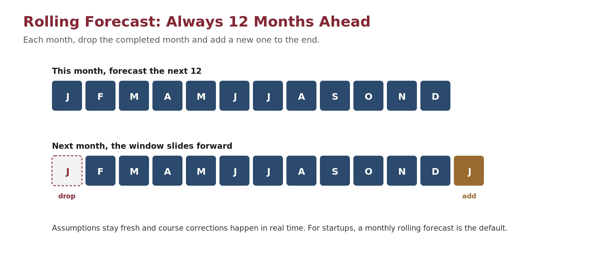
Rolling forecasts are most valuable in high-volatility and growth-stage settings, during major transitions, and anywhere a twelve-month-old assumption would be dangerously stale. For startups, a monthly rolling forecast should be the default, so assumptions stay fresh and course corrections happen in real time rather than during an annual planning cycle.
Variance Analysis Closes the Loop
A model is a hypothesis; reality is the test. Variance analysis, often called Forecast versus Actuals, compares the two. When a target is missed, the variance must be categorized to determine the response. A timing variance means the result happened in a different period than expected, such as a March payment arriving in April; no strategic change is required, only a revised timing assumption. A permanent variance means the result did not happen or the assumption was wrong, such as a cancelled contract; immediate adjustment is required.
Formula. Variance = Actual Result - Forecasted Result
The job of the finance expert is to understand the drivers of each variance, decide whether it is timing or permanent, and update the model accordingly. This feedback loop transforms a static plan into a living management tool.
Check Your Understanding
Knowledge Check 14
Forecasting & Driver-Based Models
A customer payment expected in March arrived in April. How should variance analysis classify this?
The MARCS Framework: A Unified Forecasting Workflow
Building a reliable forecast follows a sequence. MARCS is a practitioner workflow that keeps that sequence honest. It stands for Measurable, Aspirational, Realistic, Controllable, and Sequenced. The base case is built bottom-up from the controllable drivers you can influence; the aspirational target is a stretch overlay laid on top of that driver-built base, not a substitute for it.
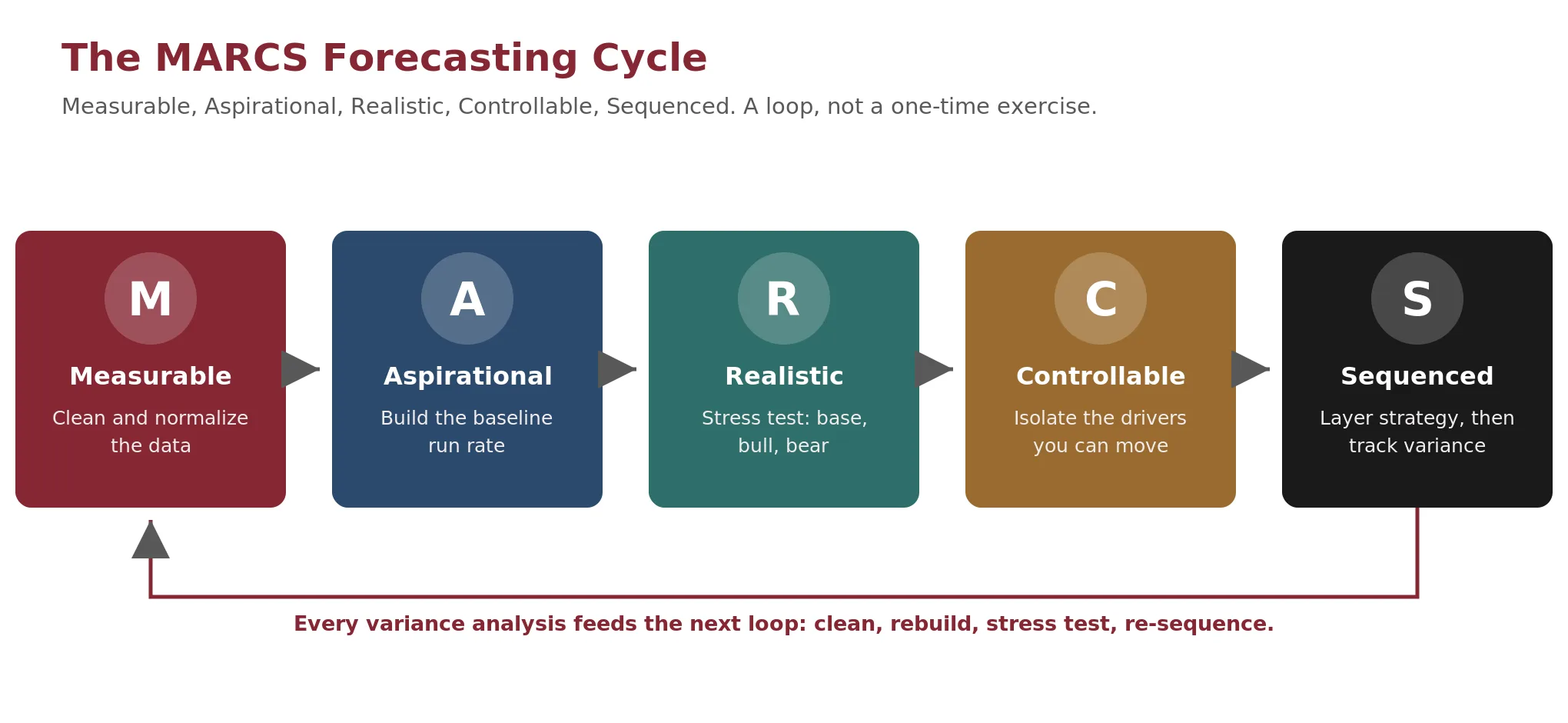
- Measurable: clean and normalize the data. Work with accurate data. Remove one-time anomalies such as lawsuit settlements or windfalls to establish an accurate baseline. For a startup with limited history, validate what you have and be explicit about where you are estimating.
- Aspirational: set the stretch target. Name the top-down ambition (where favorable execution could take the business), sized against CAGR from historical data or comparable companies. Keep it as a stretch overlay, not the operating plan: the evidence-based base case is built bottom-up from the controllable drivers below, and the aspiration is layered on top of that base rather than substituted for it.
- Realistic: stress test. Use sensitivity and scenario analysis to consider the significant outcomes. Develop base, bull, and bear cases, and pressure-test whether the aspirational targets survive contact with reality.
- Controllable: isolate the drivers and build the base case from them. Isolate the inputs that move the needle, meaning the activity, pricing, and resources you can influence rather than the market returns or macro conditions you cannot, and project the base case bottom-up from those drivers. This driver-built base case is the evidence-based foundation the aspirational target sits on top of.
- Sequenced: layer strategy and track. Adjust drivers for planned interventions, for example a certification in Q3 that supports a 15% price increase in Q4. Ensure the sequence is logical, then set a monthly or quarterly cadence to calculate variance and refresh the rolling forecast.
MARCS is not a one-time exercise. It is a cycle. Each variance analysis feeds the next iteration: clean the data, refresh the controllable drivers, rebuild the base case from them, re-test the aspirational overlay, and re-sequence the strategy. The forecast improves with every loop.
Limits of the Toolkit
Forecasting is a discipline for preparedness, not a claim of accuracy. The tools in this module structure the guesswork; they do not eliminate it.
The models assume the drivers are the right ones and the inputs are honest. For early-stage companies with little history, both are uncertain, so every output inherits that uncertainty.
The benchmarks used here, including 3:1 LTV to CAC, sub-18-month CAC payback, net revenue retention of 110 to 130%, 18 to 24 months of runway, a 1.25 to 1.4 times fully loaded cost, and a 60 to 90 day ramp, are practitioner heuristics that vary by sector, stage, and cycle.
The eleven guidelines, the sales and MRR models, and the MARCS workflow are practitioner frameworks. Lishego's guide is a self-published resource by an investment associate, useful as consensus practice rather than peer-reviewed evidence.
This module builds and stress-tests the forecast. Discounting these cash flows into a valuation is the work of Week 5, using the Gordon Growth Model.